Page 126 - Algorithm Collections for Digital Signal Processing Applications using MATLAB

114 Chapter 3

The co-efficient vector is obtained as the inner product of the vector
T(v1) with the corresponding basis.

*
T
[T(v1)] f1 = [2] [Note that the inner product complex numbers ‘a’
T
and ‘b’ is computed as a b*]

T
*
[T(v1)] f2 = [0]

T
*
[T(v1)] f1 = [ 0]

*
T
[T(v1)] f1 = [0]

Therefore the co-efficient vector associated with the vector T(v1) is
T
given as [2 0 0 0]

Similarly the co-efficient vector associated with the vector T(v2), T(v3)
T
T
T
and T(v4) is given as [0 2 0 0] , [0 0 2 0] and [0 0 0 2] respectively.

Thus the transformation matrix for the Fourier transform is given as

2 0 0 0
0 2 0 0
0 0 2 0
0 0 0 2

As the transformation matrix is the diagonal matrix with ‘2’ as the
diagonal elements, the co-efficient vector for any vector in the Vector space
1 is ‘coef’ then the co-efficient vector for the corresponding mapped vector
in the Vector space 2 (Fourier domain) is given be 2*c.

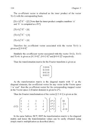
Thus the Fourier transformation of the vector [2 3 4 1] is given as the

1 1 1 1 2 * 2 10
1 -i -1 i 3 * 2 -2-i
(1/2) 1 -1 1 -1 4 *2 = 2
1 i -1 -i 1 *2 -2+2i

In the same fashion, DCT, DST the transformation matrix is the diagonal
matrix and hence the transformation values can be easily obtained using
simple matrix multiplication as described above.