Page 332 -

306 Chapter 8 ■ Classification

not to choose the same item more than once. All the items not selected will be
the training set. In principle, this can be repeated arbitrarily many times, but
nothing is gained by doing so. Between 5 and 10 trials would be sufficient for
the Iris data set. Using random cross validation, keeping the classes balanced,
and with 10 examples from each class in the test set, and overall success rate
averaged over ten trials, a 93% success rate was obtained. This would be a
little different each time due to the random nature of the experiment.
What might be called the ultimate in cross validation picks a single sample
from the entire set as test data, and uses the rest as training data. This can be
repeated for each of the samples in the set, and the average over all trials gives
the success rate. For the Iris data, there would be 150 trials, each with a single
classification. This is called leave-one-out cross validation, for obvious reasons.
For the Iris set again, leave-one-out cross validation leads to an overall
success rate of 96% when used with a nearest neighbor classifier; it’s probably
the best that can be done. This is a good technique for use with smaller data
sets, but is really too expensive for large ones.

8.4 Support Vector Machines

Section 8.1.3 discussed the concept of a linear discriminant. This is a straight
line that divides the feature values into two groups, one for each class, and is
an effective way to implement a classifier if such a line can be found. In higher
dimensional spaces — that is, if more than two features are involved — this
line becomes a plane or a hyperplane. It’s still linear, just complicated by
dimensionality. Samples that lie on one side of the plane belong to one class,
while those on the other belong to a different class. A support vector machine
(SVM) is a nitro-powered version of such a linear discriminant.
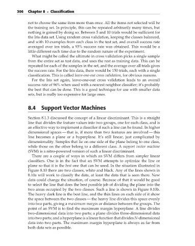
There are a couple of ways in which an SVM differs from simpler linear
classifiers. One is in the fact that an SVM attempts to optimize the line or
plane so that it is the best one that can be used. In the situation illustrated in
Figure 8.10 there are two classes, white and black. Any of the lines shown in
8.10a will work to classify the data, at least the data that is seen there. New
data could change the situation, of course. Because of that it would be good
to select the line that does the best possible job of dividing the plane into the
two areas occupied by the two classes. Such a line is shown in Figure 8.10b.
The heavy dark line is the best line, and the thin lines on each side of it show
the space between the two classes — the heavy line divides this space evenly
into two parts, giving a maximum margin or distance between the groups. The
point of an SVM is to find the maximum margin hyperplane. A line divides
two-dimensional data into two parts; a plane divides three-dimensional data
into two parts; and a hyperplane is a linear function that divides N-dimensional
data into two parts. The maximum margin hyperplane is always as far from
both data sets as possible.