Page 454 -

434 CHAPTER 10 INVENTORY MODELS

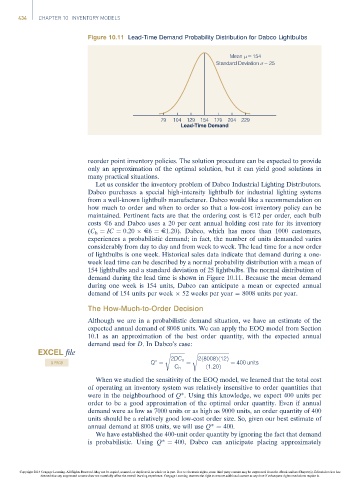
Figure 10.11 Lead-Time Demand Probability Distribution for Dabco Lightbulbs

Mean = 154
Standard Deviation = 25

79 104 129 154 179 204 229
Lead-Time Demand

reorder point inventory policies. The solution procedure can be expected to provide
only an approximation of the optimal solution, but it can yield good solutions in
many practical situations.
Let us consider the inventory problem of Dabco Industrial Lighting Distributors.
Dabco purchases a special high-intensity lightbulb for industrial lighting systems
from a well-known lightbulb manufacturer. Dabco would like a recommendation on
how much to order and when to order so that a low-cost inventory policy can be
maintained. Pertinent facts are that the ordering cost is E12 per order, each bulb
costs E6 and Dabco uses a 20 per cent annual holding cost rate for its inventory
(C h ¼ IC ¼ 0.20 E6 ¼ E1.20). Dabco, which has more than 1000 customers,
experiences a probabilistic demand; in fact, the number of units demanded varies
considerably from day to day and from week to week. The lead time for a new order
of lightbulbs is one week. Historical sales data indicate that demand during a one-
week lead time can be described by a normal probability distribution with a mean of
154 lightbulbs and a standard deviation of 25 lightbulbs. The normal distribution of
demand during the lead time is shown in Figure 10.11. Because the mean demand
during one week is 154 units, Dabco can anticipate a mean or expected annual
demand of 154 units per week 52 weeks per year ¼ 8008 units per year.

The How-Much-to-Order Decision
Although we are in a probabilistic demand situation, we have an estimate of the
expected annual demand of 8008 units. We can apply the EOQ model from Section
10.1 as an approximation of the best order quantity, with the expected annual
demand used for D. In Dabco’s case:
EXCEL file s ffiffiffiffiffiffiffiffiffiffiffiffi s ffiffiffiffiffiffiffiffiffiffiffiffiffiffiffiffiffiffiffiffiffiffiffiffiffiffi
2ð8008Þð12Þ
2DC o

Q PROB Q ¼ ¼ ¼ 400 units
C h ð1:20Þ
When we studied the sensitivity of the EOQ model, we learned that the total cost
of operating an inventory system was relatively insensitive to order quantities that
were in the neighbourhood of Q*. Using this knowledge, we expect 400 units per
order to be a good approximation of the optimal order quantity. Even if annual
demand were as low as 7000 units or as high as 9000 units, an order quantity of 400
units should be a relatively good low-cost order size. So, given our best estimate of
annual demand at 8008 units, we will use Q* ¼ 400.
We have established the 400-unit order quantity by ignoring the fact that demand
is probabilistic. Using Q* ¼ 400, Dabco can anticipate placing approximately

Copyright 2014 Cengage Learning. All Rights Reserved. May not be copied, scanned, or duplicated, in whole or in part. Due to electronic rights, some third party content may be suppressed from the eBook and/or eChapter(s). Editorial review has
deemed that any suppressed content does not materially affect the overall learning experience. Cengage Learning reserves the right to remove additional content at any time if subsequent rights restrictions require it.