Page 87 -

GENERAL LINEAR PROGRAMMING NOTATION 67

a mathematical model for a problem that involves a large number of decision
variables is much easier. For instance, for a linear programming model with three
decision variables, we would use variable names of x 1 , x 2 and x 3 ; for a problem with
four decision variables, we would use variable names of x 1 , x 2 , x 3 and x 4 and so on.
Clearly, if a problem involved 1000 decision variables, trying to identify 1000 unique
names would be difficult. However, using the general linear programming notation,
the decision variables would be defined as x 1 , x 2 , x 3 ,. . ., x 1000 .
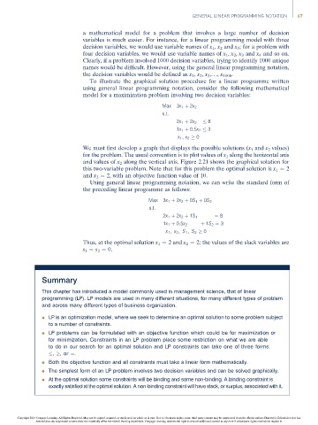
To illustrate the graphical solution procedure for a linear programme written
using general linear programming notation, consider the following mathematical
model for a maximization problem involving two decision variables:

Max 3x 1 þ 2x 2
s:t:
2x 1 þ 2x 2 8
1x 1 þ 0:5x 2 3
x 1 ; x 2 0
We must first develop a graph that displays the possible solutions (x 1 and x 2 values)
for the problem. The usual convention is to plot values of x 1 along the horizontal axis
and values of x 2 along the vertical axis. Figure 2.21 shows the graphical solution for
this two-variable problem. Note that for this problem the optimal solution is x 1 ¼ 2
and x 2 ¼ 2, with an objective function value of 10.
Using general linear programming notation, we can write the standard form of
the preceding linear programme as follows:
Max 3x 1 þ 2x 2 þ 0S 1 þ 0S 2
s:t:
¼ 8
2x 1 þ 2x 2 þ 1S 1
1x 1 þ 0:5x 2 þ 1S 2 ¼ 3
x 1 ; x 2 ; S 1 ; S 2 0
Thus, at the optimal solution x 1 ¼ 2 and x 2 ¼ 2; the values of the slack variables are
s 1 ¼ s 2 ¼ 0.

Summary

This chapter has introduced a model commonly used in management science, that of linear
programming (LP). LP models are used in many different situations, for many different types of problem
and across many different types of business organization.

l LP is an optimization model, where we seek to determine an optimal solution to some problem subject
to a number of constraints.
l LP problems can be formulated with an objective function which could be for maximization or
for minimization. Constraints in an LP problem place some restriction on what we are able
to do in our search for an optimal solution and LP constraints can take one of three forms:
, ,or ¼.
l Both the objective function and all constraints must take a linear form mathematically.
l The simplest form of an LP problem involves two decision variables and can be solved graphically.
l At the optimal solution some constraints will be binding and some non-binding. A binding constraint is
exactly satisfied at the optimal solution. A non-binding constraint will have slack, or surplus, associated with it.

Copyright 2014 Cengage Learning. All Rights Reserved. May not be copied, scanned, or duplicated, in whole or in part. Due to electronic rights, some third party content may be suppressed from the eBook and/or eChapter(s). Editorial review has
deemed that any suppressed content does not materially affect the overall learning experience. Cengage Learning reserves the right to remove additional content at any time if subsequent rights restrictions require it.