Page 159 - Analog and Digital Filter Design

1 56 Analog and Digital Filter Design

Important factors, which are related to the pole locations, are w,, and Q. The
values of these for the highpass filter are found in the same way as for the
lowpass filter. The method is repeated here. The natural frequency m,, is depend-
ent upon o, and this changes in proportion to the scaling of the diagram. The
origin to pole distance is equal to w,,. The value of Q is given by the distance
from the pole to the origin divided by twice the real coordinate. Thus Q depends
on the ratio of do. As the pole-zero diagram is scaled for a higher cutoff fre-
quency, the value of Q remains unchanged.

Now that I have set the scene, let’s take a look at some basic highpass active
filter designs and see how the pole and zero locations are used to find compo-
nent values. I shall return to the S-plane later when discussing active Cauer and
Inverse Chebyshev filters: these types both have zeroes in the stopband.

First-Order Filter Section

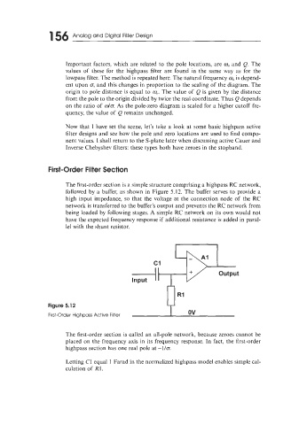
The first-order section is a simple structure comprising a highpass RC network,
followed by a buffer, as shown in Figure 5.12. The buffer serves to provide a
high input impedance, so that the voltage at the connection node of the RC
network is transferred to the buffer’s output and prevents the RC network from
being loaded by following stages. A simple RC network on its own would not
have the expected frequency response if additional resistance is added in paral-
lel with the shunt resistor.

Figure 5.12
First-Order Highpass Active Filter

The first-order section is called an all-pole network, because zeroes cannot be
placed on the frequency axis in its frequency response. In fact, the first-order
highpass section has one real pole at -1lo.

Letting C1 equal 1 Farad in the normalized highpass model enables simple cal-
culation of R l.