Page 360 - Analog and Digital Filter Design

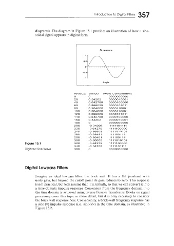
Introduction to Digital Filters 357

diagrams). The diagram in Figure 15.1 provides an illustration of how a sinu-
soidal signal appears in digital form.

Sinewave

I Angle

ANGLE SIN(x) Two's Corndement
..
0 0 0000000000
20 0.34202 000001 0001
40 0.642788 00001 00000
60 0.866025 00001 01 03 1
80 0.984808 0000170001
100 0.984808 00001 10001
120 0.866025 00001 01 01 1
140 0.642788 00001 00000
160 0.34202 000001 0001
180 0 0000000000
200 -0.34202 11111011 11
220 -0.64279 11 111 00000
240 -0.86603 111101 0101
260 -0.9848 1 11 I 001 11 1
1
280 -0.9848 11 11 001 17 1
1
300 -0.86603 11 11 010101
Figure 15.1 320 -0.64279 11 11 100000
340 -0.34202 1111101111
Digitized Sine Wave 360 0 0000000000

Digital Lowpass Filters

Imagine an ideal lowpass filter: the brick wall. It has a flat passband with
unity gain, but beyond the cutoff point its gain reduces to zero. This response
is not practical, but let's assume that it is, initially, so that we can convert it into
a time-domain impulse response. Conversion from the frequency domain into
the time domain is achieved using inverse Fourier Transforms. Books on signal
processing cover this topic in more detail, but it is only necessary to consider
the brick wall response here. Conveniently, a brick-wall frequency response has
a sinc (x) impulse response (i.e., sin(x)/x) in the time domain, as illustrated in
Figure 15.2.