Page 89 - Analog and Digital Filter Design

86 Analog and Digital Filter Design

A pole is said to exist where the transfer function would have a value of infin-
ity. This is when the denominator of the equation is equal to zero. So poles exist
at location x when ax2 + bx + c = 0.

The well-known root-finding equation: x = -bf can be used to find
2a
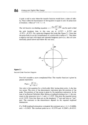
the pole locations that, in this case, are at -0.7071 + j0.7071 and
-0.7071 -j0.7071. On a pole-zero diagram this looks like Figure 3.1. Note that
the poles both lie on the circumference of a circle with a radius of 1. They have
a negative real part with equal and opposite imaginary parts (i.e., they are sym-
metrically placed above and below the real axis).

I
Figure 3.1 -’
Second-Order Pole-Zero Diagram

Now let’s consider a more complicated filter. The transfer function is given by
general expression:

ds’+e
T(w) =
as?+bs+c‘
Not only is this equation for a third-order filter having three poles, it also has
two zeroes. The roots of the denominator expression give the position of the
poles. The position of the zeroes is given by the numerator expression. In the
case of an Inverse Chebyshev filter, having a stopband starting at w= 1, the con-
stants in the numerator are d = 1 and e = 1.3333. This gives the required zeroes
at kjl.15470. Note that these are on the imaginary “j“ axis and have no “real”
part. The constants in the denominator depend on the required stopband
attenuation .

If a 30dB stopband attenuation is required the constants are a = 1, b = 0.44086,
and c = 0.23621. The resultant poles are at -0.53578 and -0.22043 kJo.43315.