Page 225 - Applied Numerical Methods Using MATLAB

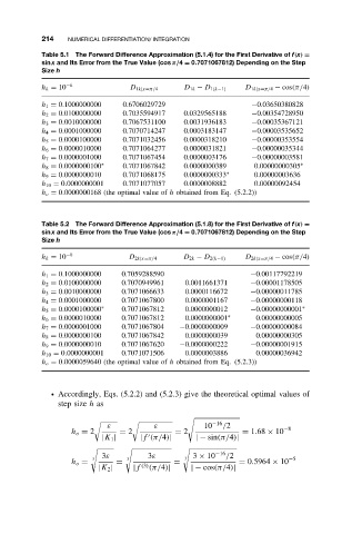
214 NUMERICAL DIFFERENTIATION/ INTEGRATION
Table 5.1 The Forward Difference Approximation (5.1.4) for the First Derivative of f(x) =
sin x and Its Error from the True Value (cos π/4 = 0.7071067812) Depending on the Step
Size h
h k = 10 −k D 1k|x=π/4 D 1k − D 1(k−1) D 1k|x=π/4 − cos(π/4)

h 1 = 0.1000000000 0.6706029729 −0.03650380828
h 2 = 0.0100000000 0.7035594917 0.0329565188 −0.00354728950
h 3 = 0.0010000000 0.7067531100 0.0031936183 −0.00035367121
h 4 = 0.0001000000 0.7070714247 0.0003183147 −0.00003535652
h 5 = 0.0000100000 0.7071032456 0.0000318210 −0.00000353554
h 6 = 0.0000010000 0.7071064277 0.0000031821 −0.00000035344
h 7 = 0.0000001000 0.7071067454 0.0000003176 −0.00000003581
h 8 = 0.0000000100 ∗ 0.7071067842 0.0000000389 0.00000000305 ∗
h 9 = 0.0000000010 0.7071068175 0.0000000333 ∗ 0.00000003636
h 10 = 0.0000000001 0.7071077057 0.0000008882 0.00000092454
h o = 0.0000000168 (the optimal value of h obtained from Eq. (5.2.2))

Table 5.2 The Forward Difference Approximation (5.1.8) for the First Derivative of f(x) =
sin x and Its Error from the True Value (cos π/4 = 0.7071067812) Depending on the Step
Size h

h k = 10 −k D 2k|x=π/4 D 2k − D 2(k−1) D 2k|x=π/4 − cos(π/4)
h 1 = 0.1000000000 0.7059288590 −0.00117792219
h 2 = 0.0100000000 0.7070949961 0.0011661371 −0.00001178505
h 3 = 0.0010000000 0.7071066633 0.0000116672 −0.00000011785
h 4 = 0.0001000000 0.7071067800 0.0000001167 −0.00000000118
h 5 = 0.0000100000 ∗ 0.7071067812 0.0000000012 −0.00000000001 ∗
h 6 = 0.0000010000 0.7071067812 0.0000000001 ∗ 0.00000000005
h 7 = 0.0000001000 0.7071067804 −0.0000000009 −0.00000000084
h 8 = 0.0000000100 0.7071067842 0.0000000039 0.00000000305
h 9 = 0.0000000010 0.7071067620 −0.0000000222 −0.00000001915
h 10 = 0.0000000001 0.7071071506 0.0000003886 0.00000036942
h o = 0.0000059640 (the optimal value of h obtained from Eq. (5.2.3))

ž Accordingly, Eqs. (5.2.2) and (5.2.3) give the theoretical optimal values of
step size h as

−16
ε ε 10 /2 −8
h o = 2 = 2 = 2 = 1.68 × 10

|K 1 | |f (π/4)| |− sin(π/4)|

3ε 3ε 3 3 × 10 −16 /2
3 3 −5
h o = = = = 0.5964 × 10
|K 2 | |f (3) (π/4)| |− cos(π/4)|