Page 230 - Applied Numerical Methods Using MATLAB

DIFFERENCE APPROXIMATION FOR SECOND AND HIGHER DERIVATIVE 219

function [c,err,eoh,A,b] = difapx(N,points)
%difapx.m to get the difference approximation for the Nth derivative
l = max(points);
L = abs(points(1)-points(2))+ 1;
ifL<N+1, error(’More points are needed!’); end
forn=1:L
A(1,n) = 1;
for m = 2:L + 2, A(m,n) = A(m - 1,n)*l/(m - 1); end %Eq.(5.3.5)
l = l-1;
end
b = zeros(L,1); b(N + 1) = 1;
c =(A(1:L,:)\b)’; %coefficients of difference approximation formula
err = A(L + 1,:)*c’; eoh = L-N; %coefficient & order of error term
if abs(err) < eps, err = A(L + 2,:)*c’; eoh=L-N +1;end
if points(1) < points(2), c = fliplr(c); end

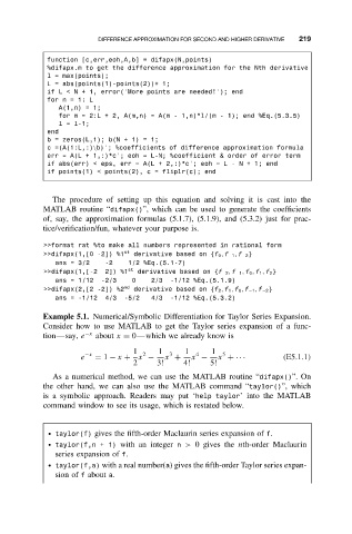
The procedure of setting up this equation and solving it is cast into the
MATLAB routine “difapx()”, which can be used to generate the coefficients
of, say, the approximation formulas (5.1.7), (5.1.9), and (5.3.2) just for prac-
tice/verification/fun, whatever your purpose is.

>>format rat %to make all numbers represented in rational form
>>difapx(1,[0 -2]) %1 st derivative based on {f 0 , f −1 , f −2 }
ans = 3/2 -2 1/2 %Eq.(5.1-7)
>>difapx(1,[-2 2]) %1 st derivative based on {f −2 , f −1 , f 0 , f 1 , f 2 }
ans = 1/12 -2/3 0 2/3 -1/12 %Eq.(5.1.9)
>>difapx(2,[2 -2]) %2 nd derivative based on {f 2 , f 1 , f 0 , f −1 , f −2 }
ans = -1/12 4/3 -5/2 4/3 -1/12 %Eq.(5.3.2)

Example 5.1. Numerical/Symbolic Differentiation for Taylor Series Expansion.
Consider how to use MATLAB to get the Taylor series expansion of a func-
tion—say, e −x about x = 0—which we already know is
1 2 1 3 1 4 1 5
−x
e = 1 − x + x − x + x − x +· · · (E5.1.1)
2 3! 4! 5!
As a numerical method, we can use the MATLAB routine “difapx()”. On
the other hand, we can also use the MATLAB command “taylor()”, which
is a symbolic approach. Readers may put ‘help taylor’ into the MATLAB
command window to see its usage, which is restated below.

ž taylor(f) gives the fifth-order Maclaurin series expansion of f.
ž taylor(f,n + 1) with an integer n > 0 gives the nth-order Maclaurin
series expansion of f.
ž taylor(f,a) with a real number(a) gives the fifth-order Taylor series expan-
sion of f about a.