Page 234 - Applied Numerical Methods Using MATLAB

NUMERICAL INTEGRATION AND QUADRATURE 223

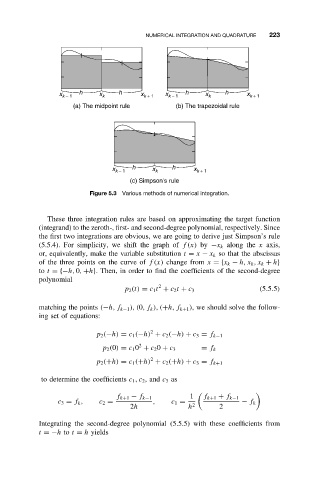
x k − 1 h x k h x k + 1 x k − 1 h x k h x k + 1
(a) The midpoint rule (b) The trapezoidal rule

x k − 1 h x k h x k + 1
(c) Simpson's rule
Figure 5.3 Various methods of numerical integration.

These three integration rules are based on approximating the target function
(integrand) to the zeroth-, first- and second-degree polynomial, respectively. Since
the first two integrations are obvious, we are going to derive just Simpson’s rule
(5.5.4). For simplicity, we shift the graph of f(x) by −x k along the x axis,
or, equivalently, make the variable substitution t = x − x k so that the abscissas
of the three points on the curve of f(x) change from x ={x k − h, x k ,x k + h}
to t ={−h, 0, +h}. Then, in order to find the coefficients of the second-degree
polynomial
2
p 2 (t) = c 1 t + c 2 t + c 3 (5.5.5)

matching the points (−h, f k−1 ), (0,f k ), (+h, f k+1 ), we should solve the follow-
ing set of equations:

2
p 2 (−h) = c 1 (−h) + c 2 (−h) + c 3 = f k−1
2
p 2 (0) = c 1 0 + c 2 0 + c 3 = f k
2
p 2 (+h) = c 1 (+h) + c 2 (+h) + c 3 = f k+1
to determine the coefficients c 1 ,c 2 ,and c 3 as

f k+1 − f k−1 1 f k+1 + f k−1
c 3 = f k , c 2 = , c 1 = − f k
2h h 2 2
Integrating the second-degree polynomial (5.5.5) with these coefficients from
t =−h to t = h yields