Page 233 - Applied Numerical Methods Using MATLAB

222 NUMERICAL DIFFERENTIATION/ INTEGRATION
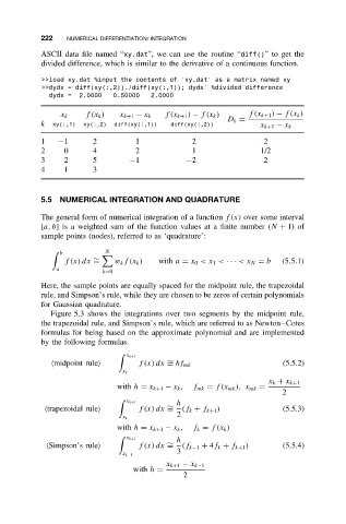
ASCII data file named “xy.dat”, we can use the routine “diff()”toget the
divided difference, which is similar to the derivative of a continuous function.
>>load xy.dat %input the contents of ’xy.dat’ as a matrix named xy
>>dydx = diff(xy(:,2))./diff(xy(:,1)); dydx’ %divided difference
dydx = 2.0000 0.50000 2.0000

f(x k ) f(x k+1 ) − f(x k ) f(x k+1 ) − f(x k )
x k x k+1 − x k
D k =
k xy(:,1) xy(:,2) diff(xy(:,1)) diff(xy(:,2)) x k+1 − x k
1 −1 2 1 2 2
2 0 4 2 1 1/2
3 2 5 −1 −2 2
4 1 3

5.5 NUMERICAL INTEGRATION AND QUADRATURE

The general form of numerical integration of a function f(x) over some interval
[a, b] is a weighted sum of the function values at a finite number (N + 1) of
sample points (nodes), referred to as ‘quadrature’:

b N

∼
f(x) dx = w k f(x k ) with a = x 0 <x 1 < ·· · <x N = b (5.5.1)
a
k=0
Here, the sample points are equally spaced for the midpoint rule, the trapezoidal
rule, and Simpson’s rule, while they are chosen to be zeros of certain polynomials
for Gaussian quadrature.
Figure 5.3 shows the integrations over two segments by the midpoint rule,
the trapezoidal rule, and Simpson’s rule, which are referred to as Newton–Cotes
formulas for being based on the approximate polynomial and are implemented
by the following formulas.
x k+1

∼
midpoint rule
f(x) dx = hf mk (5.5.2)
x k
x k + x k+1
with h = x k+1 − x k , f mk = f(x mk ), x mk =
2
h
x k+1

∼
trapezoidal rule
f(x) dx = (f k + f k+1 ) (5.5.3)
2
x k
with h = x k+1 − x k , f k = f(x k )

x k+1 h
∼
Simpson’s rule
f(x) dx = (f k−1 + 4f k + f k+1 ) (5.5.4)
3
x k−1
x k+1 − x k−1
with h =
2