Page 232 - Applied Numerical Methods Using MATLAB

INTERPOLATING POLYNOMIAL AND NUMERICAL DIFFERENTIAL 221
given only the data file containing several data points. A possible measure is
to make the interpolating function by using one of the methods explained in
Chapter 3 and get the derivative of the interpolating function.
For simplicity, let’s reconsider the problem of finding the derivative of f(x) =
sin x at x = π/4, where the function is given as one of the following data
point sets:

π π π π 3π 3π

, sin , , sin , , sin
8 8 4 4 8 8

π π π π 3π 3π 4π 4π

(0, sin 0), , sin , , sin , , sin , , sin
8 8 4 4 8 8 8 8
2π 2π 3π 3π 4π 4π 5π 5π 6π 6π

, sin , , sin , , sin , , sin , , sin
16 16 16 16 16 16 16 16 16 16
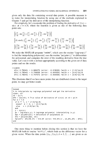
We make the MATLAB program “nm540”, which uses the routine “lagranp()”
to find the interpolating polynomial, uses the routine “polyder()” to differentiate
the polynomial, and computes the error of the resulting derivative from the true
value. Let’s run it with x defined appropriately according to the given set of data
points and see the results.
>>nm540
dfx( 0.78540) = 0.689072 (error: -0.018035) %with x = [1:3]*pi/8
dfx( 0.78540) = 0.706556 (error: -0.000550) %with x = [0:4]*pi/8
dfx( 0.78540) = 0.707072 (error: -0.000035) %with x = [2:6]*pi/16

This illustrates that if we have more points that are distributed closer to the target
point, we may get better result.

%nm540
% to interpolate by Lagrange polynomial and get the derivative
clear, clf
x0 = pi/4;
df0 = cos(x0); % True value of derivative of sin(x) at x0 = pi/4
for m = 1:3
if m == 1, x = [1:3]*pi/8;
elseif m == 2, x = [0:4]*pi/8;
else x = [2:6]*pi/16;
end
y = sin(x);
px = lagranp(x,y); % Lagrange polynomial interpolating (x,y)
dpx = polyder(px); % derivative of polynomial px
dfx = polyval(dpx, x0);
fprintf(’ dfx(%6.4f) = %10.6f (error: %10.6f)\n’, x0,dfx,dfx - df0);
end

One more thing to mention before closing this section is that we have the
MATLAB built-in routine “diff()”, which finds us the difference vector for a
given vector. When the data points {(x k ,f (x k )), k = 1, 2,...} are given as an