Page 239 - Applied Numerical Methods Using MATLAB

228 NUMERICAL DIFFERENTIATION/ INTEGRATION
5.7 RECURSIVE RULE AND ROMBERG INTEGRATION

In this section, we are going to look for a recursive formula which enables us
to use some numerical integration with the segment width h to produce another
(hopefully better) numerical integration with half the segment width (h/2). Addi-
tionally, we use Richardson extrapolation (Section 5.1) together with the two
successive numerical integrations to make a Romberg table that can be used to
improve the accuracy of the numerical integral step by step.
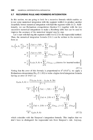
Let’s start with halving the segment width h to h/2 for the trapezoidal method.
Then, the numerical integration formula (5.6.1) can be written in the recursive
form as

2N−1
h h f(a) + f(b)
I T 2 a, b, = + f(x k/2 )
2 2 2
k=1
N−1 N−1
h f(a) + f(b)
= + f(x 2m/2 ) + f(x (2m+1)/2 )
2 2
m=1 m=0
N−1
1
= I T 2 (a,b,h) + f(x (2m+1)/2 )(terms for inserted nodes)
2
m=0
(5.7.1)
2
2
Noting that the error of this formula is proportional to h (O(h )), we apply a
Richardson extrapolation [Eq. (5.1.10)] to write a higher-level integration formula
4
having an error of O(h ) as
2
2 I T 2 (a,b,h) − I T 2 (a, b, 2h)
I T 4 (a,b,h) =
2 − 1
2
N−1
(5.6.1) 1 h
= 4 f(a) + f(b) + 2 f(x k )
3 2
k=1
N/2−1

2h
− f(a) + f(b) + 2 f(x 2m )
2
m=1
N/2 N/2−1

h
= f(a) + f(b) + 4 f(x 2m−1 ) + 2 f(x 2m )
3
m=1 m=1
(5.6.2)
≡ I S4 (a,b,h) (5.7.2)
which coincides with the Simpson’s integration formula. This implies that we
don’t have to distinguish the trapezoidal rule from Simpson’s rule. Anyway,