Page 243 - Applied Numerical Methods Using MATLAB

232 NUMERICAL DIFFERENTIATION/ INTEGRATION
the routine “adap_smpsn()”, which needs the calling routine “adapt_smpsn()”
for start-up.

function [INTf,nodes,err] = adap smpsn(f,a,b,INTf,tol,varargin)
%adaptive recursive Simpson method
c = (a+b)/2;
INTf1 = smpsns(f,a,c,1,varargin{:});
INTf2 = smpsns(f,c,b,1,varargin{:});
INTf12 = INTf1 + INTf2;
err = abs(INTf12 - INTf)/15; % Error estimate by Eq.(5.5.13)
if isnan(err) | err < tol | tol<eps % NaN? Satisfying error? Too deep level?
INTf = INTf12;
points = [a c b];
else
[INTf1,nodes1,err1] = adap smpsn(f,a,c,INTf1,tol/2,varargin{:});
[INTf2,nodes2,err2] = adap smpsn(f,c,b,INTf2,tol/2,varargin{:});
INTf = INTf1 + INTf2;
nodes = [nodes1 nodes2(2:length(nodes2))];
err = err1 + err2;
end
function [INTf,nodes,err] = adapt smpsn(f,a,b,tol,varargin)
%apply adaptive recursive Simpson method
INTf = smpsns(f,a,b,1,varargin{:});
[INTf,nodes,err] = adap smpsn(f,a,b,INTf,tol,varargin{:});

We can apply these routines to get the approximate value of integration
(5.7.5) by putting the following MATLAB statements into the MATLAB com-
mand window.

>>f = inline(’400*x.*(1 - x).*exp(-2*x)’,’x’);
>>a=0;b=4;tol= 0.001;
>>format short e
>>true I = 3200*exp(-8);
>>Ias = adapt smpsn(f,a,b,tol), erras=Ias-true I
Ias = 1.0735e+000, erras = -8.9983e-006
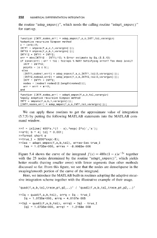
Figure 5.4 shows the curve of the integrand f(x) = 400x(1 − x)e −2x together
with the 25 nodes determined by the routine “adapt_smpsn()”, which yields
better results (having smaller error) with fewer segments than other methods
discussed so far. From this figure, we see that the nodes are dense/sparse in the
swaying/smooth portion of the curve of the integrand.
Here, we introduce the MATLAB built-in routines adopting the adaptive recur-
sive integration scheme together with the illustrative example of their usage.

"quad(f,a,b,tol,trace,p1,p2,..)" / "quadl(f,a,b,tol,trace,p1,p2,..)"

>>Iq = quad(f,a,b,tol), errq = Iq - true I
Iq = 1.0735e+000, errq = 4.0107e-005
>>Iql = quadl(f,a,b,tol), errql = Iql - true I
Iql = 1.0735e+000, errq1 = -1.2168e-008