Page 246 - Applied Numerical Methods Using MATLAB

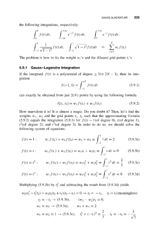
GAUSS QUADRATURE 235
the following integrations, respectively:

b +∞ 2 +∞
−t
f(t) dt, e −t f(t) dt, e f(t) dt,
a −∞ 0
N
1 1 1
2
√ f(t) dt, 1 − t f(t)dt ≈ w i f(t i )
−1 1 − t 2 −1
i=1
The problem is how to fix the weight w i ’s and the (Gauss) grid points t i ’s.
5.9.1 Gauss–Legendre Integration
If the integrand f(t) is a polynomial of degree ≤ 3(= 2N − 1), then its inte-
gration
+1
I(−1, 1) = f(t) dt (5.9.1)
−1
can exactly be obtained from just 2(N) points by using the following formula

I[t 1 ,t 2 ] = w 1 f(t 1 ) + w 2 f(t 2 ) (5.9.2)

How marvelous it is! It is almost a magic. Do you doubt it? Then, let’s find the
weights w 1 , w 2 and the grid points t 1 , t 2 such that the approximating formula
(5.9.2) equals the integration (5.9.1) for f(t) = 1(of degree 0), t(of degree 1),
3
2
t (of degree 2), and t (of degree 3). In order to do so, we should solve the
following system of equations:
1

f(t) = 1: w 1 f(t 1 ) + w 2 f(t 2 ) = w 1 + w 2 ≡ 1 dt = 2 (5.9.3a)
−1
1
f(t) = t : w 1 f(t 1 ) + w 2 f(t 2 ) = w 1 t 1 + w 2 t 2 ≡ tdt = 0 (5.9.3b)
−1
1 2
2
2
2
2
f(t) = t : w 1 f(t 1 ) + w 2 f(t 2 ) = w 1 t + w 2 t ≡ t dt = (5.9.3c)
1 2
−1 3
1
3
3
3
3
f(t) = t : w 1 f(t 1 ) + w 2 f(t 2 ) = w 1 t + w 2 t ≡ t dt = 0 (5.9.3d)
1 2
−1
2
Multiplying (5.9.3b) by t and subtracting the result from (5.9.3d) yields
1
3
2
w 2 (t − t t 2 ) = w 2 t 2 (t 2 + t 1 )(t 2 − t 1 ) = 0 → t 2 =− t 1 , t 2 = t 1 (meaningless)
2 1
t 2 =−t 1 → (5.9.3b), (w 1 − w 2 )t 1 = 0,
w 1 = w 2 → (5.9.3a), w 1 + w 1 = 2
2 1
2
2
w 1 = w 2 = 1 → (5.9.3c), t + (−t 1 ) = , t 1 =−t 2 =−√
1
3 3