Page 249 - Applied Numerical Methods Using MATLAB

238 NUMERICAL DIFFERENTIATION/ INTEGRATION
can get the integral (5.7.5) by simply putting the following statements into the
MATLAB command window. The result shows that the 10-point Gauss–Legendre
formula yields better accuracy (smaller error), even with fewer nodes/segments
than other methods discussed so far.

>>f = inline(’400*x.*(1 - x).*exp(-2*x)’,’x’); %Eq.(5.7.5)
>>format short e
>>true_I = 3200*exp(-8);
>>a=0;b=4;N=10; %integration interval & number of nodes(grid points)
>>IGL = gauss_legendre(f,a,b,N), errGL = IGL-true_I
IGL = 1.0735e+000, errGL = 1.6289e-009
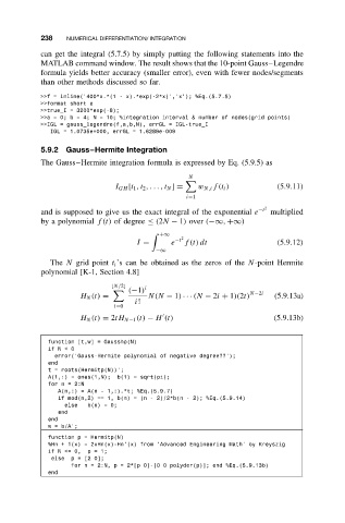
5.9.2 Gauss–Hermite Integration
The Gauss–Hermite integration formula is expressed by Eq. (5.9.5) as

N

I GH [t 1 ,t 2 ,. ..,t N ] = w N,i f(t i ) (5.9.11)
i=1
and is supposed to give us the exact integral of the exponential e −t 2 multiplied
by a polynomial f(t) of degree ≤ (2N − 1) over (−∞, +∞)
+∞ 2

I = e −t f(t) dt (5.9.12)
−∞
The N grid point t i ’s can be obtained as the zeros of the N-point Hermite
polynomial [K-1, Section 4.8]
N/2 i
(−1) N−2i
H N (t) = N(N − 1) ·· · (N − 2i + 1)(2t) (5.9.13a)
i!
i=0

H N (t) = 2tH N−1 (t) − H (t) (5.9.13b)

function [t,w] = Gausshp(N)
ifN<0
error(’Gauss-Hermite polynomial of negative degree??’);
end
t = roots(Hermitp(N))’;
A(1,:) = ones(1,N); b(1) = sqrt(pi);
for n = 2:N
A(n,:) = A(n - 1,:).*t; %Eq.(5.9.7)
if mod(n,2) == 1, b(n) = (n - 2)/2*b(n - 2); %Eq.(5.9.14)
else b(n) = 0;
end
end
w = b/A’;
function p = Hermitp(N)
%Hn + 1(x) = 2xHn(x)-Hn’(x) from ’Advanced Engineering Math’ by Kreyszig
ifN<=0, p = 1;
else p = [2 0];
for n = 2:N, p = 2*[p 0]-[0 0 polyder(p)]; end %Eq.(5.9.13b)
end