Page 247 - Applied Numerical Methods Using MATLAB

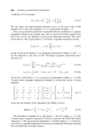
236 NUMERICAL DIFFERENTIATION/ INTEGRATION
so that Eq. (5.9.2) becomes

1 1
I[t 1 ,t 2 ] = f −√ + f √ (5.9.4)
3 3
We can expect this approximating formula to give us the exact value of the
integral (5.9.1) when the integrand f(t) is a polynomial of degree ≤ 3.
Now, you are concerned about how to generalize this two-point Gauss–Legendre
integration formula to an N-point case, since a system of nonlinear equation like
Eq. (5.9.3) can be very difficult to solve as the dimension increases. But, don’t
worry about it. The N grid points (t i ’s) of Gauss–Legendre integration formula

N

I GL [t 1 ,t 2 ,...,t N ] = w N,i f(t i ) (5.9.5)
i=1
giving us the exact integral of an integrand polynomial of degree ≤ (2N − 1)
can be obtained as the zeros of the Nth-degree Legendre polynomial [K-1,
Section 4.3]

N/2
i (2N − 2i)! N−2i
L N (t) = (−1) t (5.9.6a)
N
2 i!(N − i)!(N − 2i)!
i=0
1
L N (t) = ((2N − 1)tL N−1 (t) − (N − 1)L N−2 (t)) (5.9.6b)
N
Given the N grid point t i ’s, we can get the corresponding weight w N,i ’s of the
N-point Gauss–Legendre integration formula by solving the system of linear
equations

   
1 1 1 ž 1  w N,1  2
 t 1 t 2 t n ž t N   0 
 w N,2 
 n−1 t n−1 t n−1 ž t n−1     n  (5.9.7)


t
 w N,n  =
 (1 − (−1) )/n 
 1 2 n N   
ž ž ž ž  ž  ž
 ž   
N
t N−1 t N−1 t N−1 ž t N−1 w N,N (1 − (−1) )/N
1 2 n N
where the nth element of the right-hand side (RHS) vector is
1
1 1 − (−1) n
t
RHS(n) = t n−1 dt = 1 = (5.9.8)
n
−1 n −1 n
This procedure of finding the N grid point t i ’s and the weight w N,i ’s of the
N-point Gauss–Legendre integration formula is cast into the MATLAB routine
“Gausslp()”. We can get the two grid point t i ’s and the weight w N,i ’s of the two-
point Gauss–Legendre integration formula by just putting the following statement
into the MATLAB command window.