Page 248 - Applied Numerical Methods Using MATLAB

GAUSS QUADRATURE 237

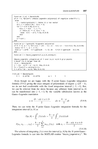
function [t,w] = Gausslp(N)
ifN<0, fprintf(’\nGauss-Legendre polynomial of negative order??\n’);
else
t = roots(Lgndrp(N))’; %make it a row vector
A(1,:) = ones(1,N); b(1) = 2;
for n = 2:N % Eq.(5.9.7)
A(n,:) = A(n - 1,:).*t;
if mod(n,2) == 0, b(n) = 0;
else b(n) = 2/n; % Eq.(5.9.8)
end
end
w = b/A’;
end
function p = Lgndrp(N) %Legendre polynomial
ifN<=0,p=1; %n*Ln(t) = (2n - 1)t Ln - 1(t)-(n - 1)Ln-2(t) Eq.(5.9.6b)
elseif N == 1, p = [1 0];
else p = ((2*N - 1)*[Lgndrp(N - 1) 0]-(N - 1)*[0 0 Lgndrp(N - 2)])/N;
end
function I = Gauss_Legendre(f,a,b,N,varargin)

%Gauss_Legendre integration of f over [a,b] with N grid points
% Never try N larger than 25
[t,w] = Gausslp(N);
x = ((b - a)*t + a + b)/2; %Eq.(5.9.9)
fx = feval(f,x,varargin{:});
I = w*fx’*(b - a)/2; %Eq.(5.9.10)

>>[t,w] = Gausslp(2)
t = 0.5774 -0.5774 w = 1 1

Even though we are happy with the N-point Gauss–Legendre integration
formula (5.9.1) giving the exact integral of polynomials of degree ≤ (2N − 1),
we do not feel comfortable with the fixed integration interval [−1, +1]. But,
we can be relieved from the stress because any arbitrary finite interval [a, b]
can be transformed into [−1, +1] by the variable substitution known as the
Gauss–Legendre translation

(b − a)t + a + b b − a
x = , dx = dt (5.9.9)
2 2
Then, we can write the N-point Gauss–Legendre integration formula for the
integration interval [a, b]as

b 1
b − a
I[a, b] = f(x) dx = f(x(t)) dt
a 2 −1
N
b − a (b − a)t i + a + b
I[x 1 ,x 2 ,...,x N ] = w N,i f(x i ) with x i =
2 2
i=1
(5.9.10)
The scheme of integrating f(x) over the interval [a, b]bythe N-point Gauss–
Legendre formula is cast into the MATLAB routine “Gauss_Legendre()”. We