Page 252 - Applied Numerical Methods Using MATLAB

DOUBLE INTEGRAL 241
The N grid point t i ’s and the corresponding weight w N,i ’s are

iπ π 2 iπ
t i = cos , w N,i = sin for i = 1, 2,...,N
N + 1 N + 1 N + 1
(5.9.26)

5.10 DOUBLE INTEGRAL

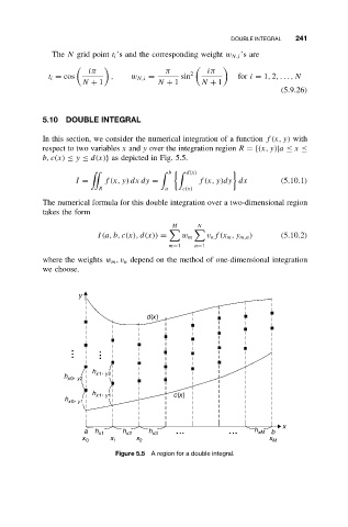
In this section, we consider the numerical integration of a function f (x, y) with
respect to two variables x and y over the integration region R ={(x, y)|a ≤ x ≤
b, c(x) ≤ y ≤ d(x)} as depicted in Fig. 5.5.

b d(x)
I = f (x, y) dx dy = f (x, y)dy dx (5.10.1)
R a c(x)
The numerical formula for this double integration over a two-dimensional region
takes the form
M N

I(a, b, c(x), d(x)) = w m v n f(x m ,y m,n ) (5.10.2)
m=1 n=1
where the weights w m ,v n depend on the method of one-dimensional integration
we choose.

y

d(x)

h ,
h , x1 y2
x0 y2
h , c(x)
x1 y1
h ,
x0 y1
x
a h x1 h x2 h x3 h xM b
x x x x
0 1 2 M
Figure 5.5 A region for a double integral.