Page 257 - Applied Numerical Methods Using MATLAB

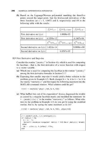
246 NUMERICAL DIFFERENTIATION/ INTEGRATION
(b) Based on the Lagrange/Newton polynomial matching the three/five
points around the target point, find the first/second derivatives of the
three functions (at x = 1, 1.0472 and 0, respectively) and fill in the
following table with the results.

f (x)| x=1 f (x)| x=1.0472 f (x)| x=0
1 2 3
First derivative on l 2 (x) 1.0000e-03
First derivative on l 4 (x) 4.3201e-12 4.1667e-04
(2) (2) (2)
f (x)| x=1 f (x)| x=1.0472 f
1 2 3 (x)| x=0
Second derivative on l 2 (x) 1.4211e-14 0.0000e+00
Second derivative on l 4 (x) 6.8587e-03

5.3 First Derivative and Step-size

Consider the routine “jacob()” in Section 4.6, which is used for computing
the Jacobian—that is, the first derivative of a vector function with respect
to a vector variable.
(a) Which one is used for computing the Jacobian in the routine “jacob()”
among the first derivative formulas in Section 5.1?
(b) Expecting that smaller step-size h would yield a better solution to the
problem given in Example 4.3, Bush changed h = 1e-4 to h = 1e-5 in
the routine “newtons()” and then typed the following statement into the
MATLAB command window. What solution could he get?

>>rn1 = newtons(’phys’,1e6,1e-4,100)
(c) What baffled him out of his expectation? Jessica diagnosed the trouble
as caused by a singular Jacobian matrix and modified the statement ‘dx
= -jacob()\fx(:)’ in the routine “newtons()” as follows. What solu-
tion (to the problem in Example 4.3) do you get by using the modified
routine, that is, by typing the same statement as in (b)?

>>rn2 = newtons(’phys’,1e6,1e-4,100), phys(rn2)

J = jacob(f,xx(k,:),h,varargin{:});
if rank(J) < Nx
k=k-1;
fprintf(’Jacobian singular! det(J) = %12.6e\n’,det(J)); break;
else
dx=-J\fx(:); %-[dfdx]^-1*fx;
end