Page 260 - Applied Numerical Methods Using MATLAB

PROBLEMS 249
What are the results? Will it be better if you make the lower-bound of
the integration interval closer to zero (0), without increasing the number
of segments or (equivalently) decreasing the segment width? How about
increasing the number of segments without making the lower bound
of the integration interval closer to the original lower-bound which is
zero (0)?
(c) For the purpose of improving the performance of “adap_smpsn()”,
Vania would put the following statements into both of the routines
“smpsns()”and “adap_smpsn()”. Supplement the routines and check
whether her idea works or not.

EPS = 1e-12; fa = feval(f,a,varargin{:});
if isnan(fa)|abs(fa) == inf, a = a + max(abs(a)*EPS,EPS); end
fb = feval(f,b,varargin{:});
?? ??????????????? ?? ????? ? ?? ? ? ???????????????????? ???

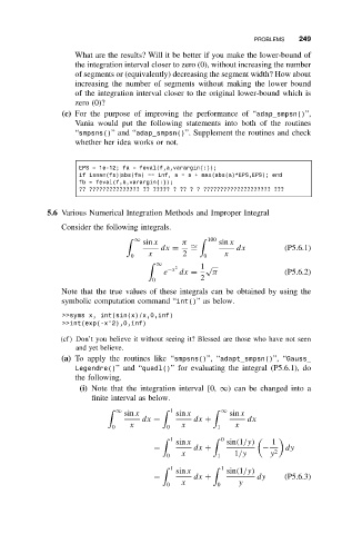
5.6 Various Numerical Integration Methods and Improper Integral
Consider the following integrals.
sin x π sin x
100
∞
dx = ∼ dx (P5.6.1)
=
x 2 x
0 0

∞ 2 1√
e −x dx = π (P5.6.2)
0 2
Note that the true values of these integrals can be obtained by using the
symbolic computation command “int()”asbelow.
>>syms x, int(sin(x)/x,0,inf)
>>int(exp(-x^2),0,inf)
(cf) Don’t you believe it without seeing it? Blessed are those who have not seen
and yet believe.
(a) To apply the routines like “smpsns()”, “adapt_smpsn()”, “Gauss_
Legendre()”and “quadl()” for evaluating the integral (P5.6.1), do
the following.
(i) Note that the integration interval [0, ∞) can be changed into a
finite interval as below.
∞ ∞
1
sin x sin x sin x
dx = dx + dx
x x x
0 0 1
sin x sin(1/y) 1
1 0
= dx + − dy
0 x 1 1/y y 2
1 1
sin x sin(1/y)

= dx + dy (P5.6.3)
x y
0 0