Page 263 - Applied Numerical Methods Using MATLAB

252 NUMERICAL DIFFERENTIATION/ INTEGRATION
“Gauss_Hermite()” works (perfectly, badly) just with two grid
points for (P5.6.2). It is because the integrand function of (P5.6.1)
is (far from, just like) a polynomial, while (P5.6.2) matches
Eq. (5.9.11) and the part of it excluding e −x 2 is (just like, far
from) a polynomial.

function I = Gauss_Hermite(f,N,varargin)
[t,w]=???????(N);
ft = feval(f,t,varargin{:});
I = w*ft’;

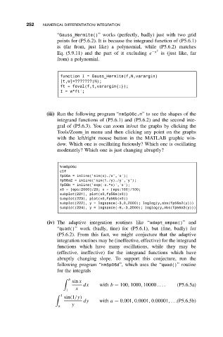
(iii) Run the following program “nm5p06c.m” to see the shapes of the
integrand functions of (P5.6.1) and (P5.6.2) and the second inte-
gral of (P5.6.3). You can zoom in/out the graphs by clicking the
Tools/Zoom in menu and then clicking any point on the graphs
with the left/right mouse button in the MATLAB graphic win-
dow. Which one is oscillating furiously? Which one is oscillating
moderately? Which one is just changing abruptly?

%nm5p06c
clf
fp56a = inline(’sin(x)./x’,’x’);
fp56a2 = inline(’sin(1./y)./y’,’y’);
fp56b = inline(’exp(-x.*x)’,’x’);
x0 = [eps:2000]/20; x = [eps:100]/100;
subplot(221), plot(x0,fp56a(x0))
subplot(223), plot(x0,fp56b(x0))
subplot(222), y = logspace(-3,0,2000); loglog(y,abs(fp56a2(y)))
subplot(224), y = logspace(-6,-3,2000); loglog(y,abs(fp56a2(y)))

(iv) The adaptive integration routines like “adapt smpsn()”and
“quad()” work (badly, fine) for (P5.6.1), but (fine, badly) for
(P5.6.2). From this fact, we might conjecture that the adaptive
integration routines may be (ineffective, effective) for the integrand
functions which have many oscillations, while they may be
(effective, ineffective) for the integrand functions which have
abruptly changing slope. To support this conjecture, run the
following program “nm5p06d”, which uses the “quad()” routine
for the integrals

b
sin x
dx with b = 100, 1000, 10000 .... (P5.6.5a)
x
1
1
sin(1/y)

dy with a = 0.001, 0.0001, 0.00001,...(P5.6.5b)
y
a