Page 266 - Applied Numerical Methods Using MATLAB

PROBLEMS 255
(i) From the fact that the Gauss–Legendre integration scheme worked
best only for (1), it is implied that the scheme is (recommendable,
not recommendable) for the case where the integrand function is
far from being approximated by a polynomial.
(ii) From the fact that the Gauss–Laguerre integration scheme worked
best only for (9), it is implied that the scheme is (recommendable,
not recommendable) for the case where the integrand function
excluding the multiplying term e −x is far from being approximated
by a polynomial.
(iii) Note the following:
ž The integrals (3) and (4) can be converted into each other by a
−1
variable substitution of x = u , dx =−u −2 du. The integrals
(5) and (6) have the same relationship.
ž The integrals (7) and (8) can be converted into each other by a
−1
variable substitution of u = e −x , dx =−u du.
From the results for (3)–(8), it can be conjectured that the numerical integra-
tion may work (better, worse) if the integration interval is changed from [1, ∞)
into (0,1] through the substitution of variable like
−n
x = u ,dx =−nu −(n+1) du or u = e −nx ,dx =−(nu) −1 du (P5.9.1)

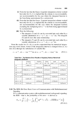
Table P5.9 The Relative Error Results of Applying Various Numerical
Integration Methods
Simpson Adaptive Gauss quad quadl
4
−6
−6
−6
(N = 10 ) (tol = 10 ) (N = 10) (tol = 10 ) (tol = 10 )
(1) 1.9984e-15 0.0000e+00 7.5719e-11
(2) 2.8955e-08 1.5343e-06
−4
(3) 9.7850e-02 (a = 10 ) 1.2713e-01 2.2352e-02
(4), b = 10 4 9.7940e-02 9.7939e-02
−4
(5) 1.2702e-02 (a = 10 ) 3.5782e-02 2.6443e-07
(6), b = 10 3 4.0250e-02 4.0250e-02
(7) 6.8678e-05 5.1077e-04 3.1781e-07
(8), b = 10 1.6951e-04 1.7392e-04
(9), b = 10 7.8276e-04 2.9237e-07 7.8276e-04

5.10 The BER (Bit Error Rate) Curve of Communication with Multidimensional
Signaling
For a communication system with multidimensional (orthogonal) signaling,
the BER—that is, the probability of bit error—is derived as
2 b−1 1 ∞ √ √ 2
P e,b = 1 − √ (Q M−1 (− 2y − bSNR))e −y dy
b
2 − 1 π −∞
(P5.10.1)