Page 268 - Applied Numerical Methods Using MATLAB

PROBLEMS 257
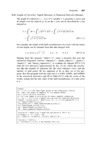
5.11 Length of Curve/Arc: Superb Harmony of Numerical Derivative/Integral.
The graph of a function y = f(x) of a variable x is generally a curve and
its length over the interval [a, b]onthe x-axis can be described by a line
integral as

b
b b
2 2 2
I = dl = dx + dy = 1 + (dy/dx) dx
a a a
b
2

= 1 + (f (x)) dx (P5.11.1)
a
For example, the length of the half-circumference of a circle with the radius
of unit length can be obtained from this line integral with

2
y = f(x) = 1 − x , a =−1, b = 1 (P5.11.2)
Starting from the program “nm5p11.m”, make a program that uses the
numerical integration routines “smpsns()”, “adapt_smpsn()”, “quad()”,
“quadl()”, and “Gauss_Legendre()” to evaluate the integral (P5.11.1,2)
with the first derivative approximated by Eq. (5.1.8), where the parame-
ters like the number of segments (N), the error tolerance (tol), and the
number of grid points (M) are supposed to be as they are in the pro-
gram. Run the program with the step size h = 0.001, 0.0001, and 0.00001
in the numerical derivative and fill in Table P5.11 with the errors of the
results, noting that the true value of the half-circumference of a unit circle
is π.

%nm5p11
a=-1;b=1;%the lower/upper bounds of the integration interval
N = 1000 % the number of segments for the Simpson method
tol = 1e-6 % the error tolerance
M = 20 % the number of grid points for Gauss–Legendre integration
IT = pi; h = 1e-3 % true integral and step size for numerical derivative
flength = inline(’sqrt(1 + dfp511(x,h).^2)’,’x’,’h’);%integrand P5.11.1)
Is = smpsns(flength,a,b,N,h);
[Ias,points,err] = adapt_smpsn(flength,a,b,tol,h);
Iq = quad(flength,a,b,tol,[],h);
Iql = quadl(flength,a,b,tol,[],h);
IGL = Gauss_Legendre(flength,a,b,M,h);
function df = dfp511(x,h) % numerical derivative of (P5.11.2)
if nargin < 2, h = 0.001; end
df = (fp511(x + h)-fp511(x - h))/2/h; %Eq.(5.1.8)
function y = fp511(x)
y = sqrt(max(1-x.*x,0)); % the function (P5.11.2)