Page 264 - Applied Numerical Methods Using MATLAB

PROBLEMS 253

%nm5p06d
fp56a = inline(’sin(x)./x’,’x’);
fp56a2 = inline(’sin(1./y)./y’,’y’);
syms x
IT2 = pi/2 - double(int(sin(x)/x,0,1)) %true value of the integral
disp(’Change of upper limit of the integration interval’)
a = 1; b = [100 1e3 1e4 1e7]; tol = 1e-4;
for i = 1:length(b)
Iq2 = quad(fp56a,a,b(i),tol);
fprintf(’With b = %12.4e, err_Iq = %12.4e\n’, b(i),Iq2-IT2);
end
disp(’Change of lower limit of the integration interval’)
a2 = [1e-3 1e-4 1e-5 1e-6 0]; b2 = 1; tol = 1e-4;
for i = 1:5
Iq2 = quad(fp56a2,a2(i),b2,tol);
fprintf(’With a2=%12.4e, err_Iq=%12.4e\n’, a2(i),Iq2-IT2);
end

Does the “quad()” routine work stably for (P5.6.5a) with the
changing value of the upper-bound of the integration interval?
Does it work stably for (P5.6.5b) with the changing value of the
lower-bound of the integration interval? Do the results support or
defy the conjecture?
(cf) This problem warns us that it may be not good to use only one routine
for a computational work and suggests us to use more than one method
for cross check.
5.7 Gauss–Hermite Integration Method
Consider the following integral:
√
∞ 2 π

e −x cos xdx = e −1/4 (P5.7.1)
0 2
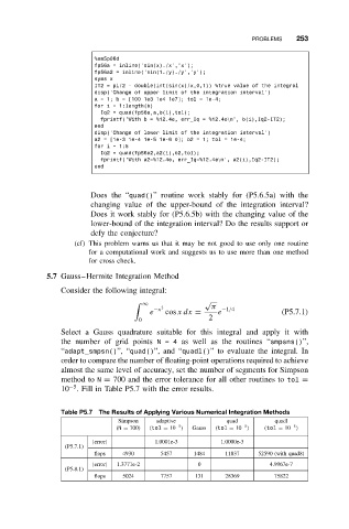
Select a Gauss quadrature suitable for this integral and apply it with
the number of grid points N=4 as well as the routines “smpsns()”,
“adapt_smpsn()”, “quad()”, and “quadl()” to evaluate the integral. In
order to compare the number of floating-point operations required to achieve
almost the same level of accuracy, set the number of segments for Simpson
method to N = 700 and the error tolerance for all other routines to tol =
−5
10 . Fill in Table P5.7 with the error results.
Table P5.7 The Results of Applying Various Numerical Integration Methods
Simpson adaptive quad quadl
−5
−5
−5
(N = 700) (tol = 10 ) Gauss (tol = 10 ) (tol = 10 )
|error| 1.0001e-3 1.0000e-3
(P5.7.1)
flops 4930 5457 1484 11837 52590 (with quad8)
|error| 1.3771e-2 0 4.9967e-7
(P5.8.1)
flops 5024 7757 131 28369 75822