Page 262 - Applied Numerical Methods Using MATLAB

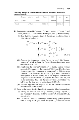
PROBLEMS 251
Table P5.6 Results of Applying Various Numerical Integration Methods for
Improper Integrals

Simpson adaptive quad Gauss S&S a&a q&q
(P5.6.1) 8.5740e-3 1.9135e-1 1.1969e+0 2.4830e-1
(P5.6.2) 6.6730e-6 0.0000e+0 3.3546e-5

(b) To apply the routines like “smpsns()”, “adapt_smpsn()”, “quad()”, and
“Gauss_Hermite()”forevaluatingtheintegral(P5.6.2),dothefollowing.
(i) Note that the integration interval [0, ∞) can be changed into a
finite interval as below.
∞ 2 2 ∞ 2
1
e −x dx = e −x dx + e −x dx
0 0 1
1 0
2 2 1
= e −x dx + e −1/y − 2 dy
0 1 y
1 2 1 e −1/y 2
= e −x dx + 2 dy (P5.6.4)
0 0 y
(ii) Compose the incomplete routine “Gauss_Hermite” like “Gauss_
Legendre”, which performs the Gauss–Hermite integration intro-
duced in Section 5.9.2.
(iii) Supplement the program “nm5p06b.m” so that the various routines
are applied for computing the integrals (P5.6.2) and (P5.6.4), where
the parameters like the number of segments (N = 200), the error
tolerance (tol = 1e-4) and the number of grid points (MGH = 2)
are supposed to be used as they are in the program. Note that the
integration interval is not (−∞, ∞) like that of Eq. (5.9.12), but
[0, ∞) and so you should cut the result of “Gauss_Hermite()”by
half to get the right answer for the integral (P5.6.2).
(iv) Run the supplemented program and fill in Table P5.6 with the
absolute errors of the results.
(c) Based on the results listed in Table P5.6, answer the following questions:
(i) Among the routines “smpsns()”, “adapt_smpsn()”, “quad()”,
and “Gauss()”, choose the best two ones for (P5.6.1) and (P5.6.2),
respectively.
(ii) The routine “Gauss–Legendre()” works (badly, perfectly) even
with as many as 20 grid points for (P5.6.1), while the routine