Page 265 - Applied Numerical Methods Using MATLAB

254 NUMERICAL DIFFERENTIATION/ INTEGRATION
5.8 Gauss–Laguerre Integration Method
(a) As in Section 5.9.1, Section 5.9.2, and Problem 5.6(b), compose the
MATLAB routines: “Laguerp()”, which generates the Laguerre poly-
nomial (5.9.18); “Gausslgp()”, which finds the grid point t i ’s and the
coefficient w N,i ’s for Gauss–Laguerre integration formula (5.9.16); and
“Gauss_Laguerre(f,N)”, which uses these two routines to carry out
the Gauss–Laguerre integration method.
(b) Consider the following integral:
∞ ∞ ∞ ∞

−t −t
−t
e tdt =−e t + e dt =−e = 1 (P5.8.1)
−t
0 0 0 0
Noting that, since this integral matches Eq. (5.9.17) with f(t) =
t, Gauss–Laguerre method is the right choice, apply the routine
“Gauss_Laguerre(f,N)” (manufactured in (a)) with N = 2as wellas
the routines “smpsns()”, “adapt_smpsn()”, “quad()”, and “quadl()”
for evaluating the integral and fill in Table P5.7 with the error results.
Which turns out to be the best? Is the performance of “quad()”
improved by lowering the error tolerance?
(cf) This illustrates that the routine “adapt_smpsn()” sometimes outperforms the
MATLAB built-in routine “quad()” with fewer computations. On the other
hand, Table P5.7 shows that it is most desirable to apply the Gauss quadrature
schemes only if one of them is applicable to the integration problem.
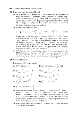
5.9 Numerical Integrals
Consider the following integrals.
π/2 1 1 2
(1) x sin xdx = 1 (2) x ln(sin x) dx =− π ln 2
0 0
2
1 1
1 ∞
(3) dx = 1 (4) dx = 1
0 x(1 − ln x) 2 1 x(1 + ln x) 2
1 π 1 π
1 ∞
(5) √ dx = (6) √ dx =
0 1
x(1 + x) 2 x(1 + x) 2
√ √

1 π π
1 ∞ √ −x
(7) ln dx = (8) xe dx =
0 0
x 2 2
1
∞ 2 −x
(9) x e cos xdx =−
0
2
4
(a) Apply the integration routines “smpsns()” (with N = 10 ), “adapt_
−6
smpsn()”, “quad()”, “quadl()”(tol = 10 )and “Gauss_leg-
endre()” (Section 5.9.1) or “Gauss_Laguerre()” (Problem 5.8) (with
N = 15) to compute the above integrals and fill in Table P5.9 with the
relative errors. Use the upper/lower bounds of the integration interval in
Table P5.9 if they are specified in the table.
(b) Based on the results listed in Table P5.9, answer the following questions
or circle the right answer.