Page 267 - Applied Numerical Methods Using MATLAB

256 NUMERICAL DIFFERENTIATION/ INTEGRATION
b
where b is the number of bits, M = 2 is the number of orthogonal wave-
forms, SNR is the signal-to-noise-ratio, and Q(·) is the error function
defined by
1 ∞ −y /2
2
Q(x) = √ e dy (P5.10.2)
2π x
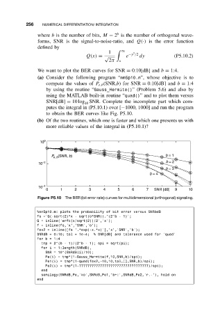
We want to plot the BER curves for SNR = 0:10[dB] and b = 1:4.
(a) Consider the following program “nm5p10.m”, whose objective is to
compute the values of P e,b (SNR,b)for SNR = 0:10[dB] and b = 1:4
by using the routine “Gauss_Hermite()” (Problem 5.6) and also by
using the MATLAB built-in routine “quad()” and to plot them versus
SNR[dB] = 10 log SNR. Complete the incomplete part which com-
10
putes the integral in (P5.10.1) over [−1000, 1000] and run the program
to obtain the BER curves like Fig. P5.10.
(b) Of the two routines, which one is faster and which one presents us with
more reliable values of the integral in (P5.10.1)?

10 0

P e, b (SNR, b) b = 1
10 −2 b = 2
b = 3
b = 4

10 −4
0 1 2 3 4 5 6 7 SNR [dB] 9 10
Figure P5.10 The BER (bit error rate) curves for multidimensional (orthogonal) signaling.

%nm5p10.m: plots the probability of bit error versus SNRbdB
fs =’Q(-sqrt(2)*x - sqrt(b*SNR)).^(2^b - 1)’;
Q = inline(’erfc(x/sqrt(2))/2’,’x’);
f = inline(fs,’x’,’SNR’,’b’);
fex2 = inline([fs ’.*exp(-x.*x)’],’x’,’SNR’,’b’);
SNRdB = 0:10; tol = 1e-4; % SNR[dB] and tolerance used for ’quad’
for b = 1:4
tmp = 2^(b - 1)/(2^b - 1); spi = sqrt(pi);
for i = 1:length(SNRdB),
SNR = 10^(SNRdB(i)/10);
Pe(i) = tmp*(1-Gauss_Hermite(f,10,SNR,b)/spi);
Pe1(i) = tmp*(1-quad(fex2,-10,10,tol,[],SNR,b)/spi);
Pe2(i) = tmp*(1-?????????????????????????????????)/spi);
end
semilogy(SNRdB,Pe,’ko’,SNRdB,Pe1,’b+:’,SNRdB,Pe2,’r.-’), hold on
end