Page 269 - Applied Numerical Methods Using MATLAB

258 NUMERICAL DIFFERENTIATION/ INTEGRATION
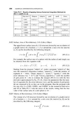
Table P5.11 Results of Applying Various Numerical Integration Methods for
(P5.11.1,2)/(P5.12.1,2)
Step-size h Simpson Adaptive quad quadl Gauss
0.001 4.6212e-2 2.9822e-2 8.4103e-2
(P5.11.1,2)
0.0001 9.4278e-3 9.4277e-3
0.00001 2.1853e-1 2.9858e-3 8.4937e-2
0.001 1.2393e-5 1.3545e-5
(P5.12.1,2)
0.0001 8.3626e-3 5.0315e-6 6.4849e-6
0.00001 1.3846e-9 8.8255e-7
(P5.13.1) N/A 8.8818e-16 0 8.8818e-16

5.12 Surface Area of Revolutionary 3-D (Cubic) Object
The upper/lower surface area of a 3-D structure formed by one revolution of
a graph (curve) of a function y = f(x) around the x-axis over the interval
[a, b] can be described by the following integral:

b b

2
I = 2π ydl = 2π f(x) 1 + (f (x)) dx (P5.12.1)

a a
For example, the surface area of a sphere with the radius of unit length can
be obtained from this equation with

2
y = f(x) = 1 − x , a =−1, b = 1 (P5.12.2)
Starting from the program “nm5p11.m”, make a program “nm5p12.m”that
uses the numerical integration routines “smpsns()” (with the number of
segments N = 1000), “adapt_smpsn()”, “quad()”, “quadl()” (with the
−6
error tolerance tol=10 )and “Gauss_Legendre()” (with the number
of grid points M=20) to evaluate the integral (P5.12.1,2) with the first
derivative approximated by Eq. (5.1.8), where the parameters like the num-
ber of segments (N), the error tolerance (tol), and the number of grid points
(M) are supposed to be as they are in the program. Run the program with
the step size h = 0.001, 0.0001, and 0.00001 in the numerical derivative
and fill in Table P5.11 with the errors of the results, noting that the true
value of the surface area of a unit sphere is 4π .
5.13 Volume of Revolutionary 3-D (Cubic) Object
The volume of a 3-D structure formed by one revolution of a graph (curve)
of a function y = f(x) around the x-axis over the interval [a, b]can be
described by the following integral:

b
2
I = π f (x) dx (P5.13.1)
a