Page 259 - Applied Numerical Methods Using MATLAB

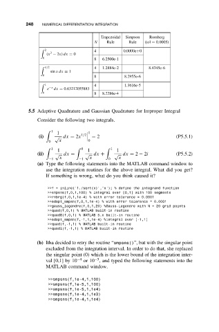
248 NUMERICAL DIFFERENTIATION/ INTEGRATION

Trapezoidal Simpson Romberg
N Rule Rule (tol = 0.0005)
2 4 0.0000e+0
3
(x − 2x) dx = 0
0 8 6.2500e-1
π/2 4 1.2884e-2 8.4345e-6
sin xdx = 1
0 8 8.2955e-6
1 4 1.3616e-5

e −x dx = 0.63212055883
0 8 8.2286e-4

5.5 Adaptive Quadrature and Gaussian Quadrature for Improper Integral

Consider the following two integrals.

1 1 1
(i) √ dx = 2x 1/2 = 2 (P5.5.1)
0 x 0
1 1 0 1 1 1
(ii) √ dx = √ dx + √ dx = 2 − 2i (P5.5.2)
−1 x −1 x 0 x
(a) Type the following statements into the MATLAB command window to
use the integration routines for the above integral. What did you get?
If something is wrong, what do you think caused it?

>>f = inline(’1./sqrt(x)’,’x’); % define the integrand function
>>smpsns(f,0,1,100) % integral over [0,1] with 100 segments
>>rmbrg(f,0,1,1e-4) % with error tolerance = 0.0001
>>adapt_smpsn(f,0,1,1e-4) % with error tolerance = 0.0001
>>gauss_legendre(f,0,1,20) %Gauss-Legendre withN=20 grid points
>>quad(f,0,1) % MATLAB built-in routine
>>quad8(f,0,1) % MATLAB 5.x built-in routine
>>adapt_smpsn(f,-1,1,1e-4) %integral over [-1,1]
>>quad(f,-1,1) % MATLAB built-in routine
>>quadl(f,-1,1) % MATLAB built-in routine

(b) Itha decided to retry the routine “smpsns()”, but with the singular point
excluded from the integration interval. In order to do that, she replaced
the singular point (0) which is the lower bound of the integration inter-
−5
val [0,1] by 10 −4 or 10 , and typed the following statements into the
MATLAB command window.

>>smpsns(f,1e-4,1,100)
>>smpsns(f,1e-5,1,100)
>>smpsns(f,1e-5,1,1e4)
>>smpsns(f,1e-4,1,1e3)
>>smpsns(f,1e-4,1,1e4)