Page 244 - Applied Numerical Methods Using MATLAB

ADAPTIVE QUADRATURE 233
(cf) These routines are capable of passing the parameters (p1,p2,..) to the integrand
(target) function and can be asked to show a list of intermediate subintervals with
the fifth input argument trace=1.
(cf) quadl() is introduced in MATLAB 6.x version to replace another adaptive integration
routine quad8() which is available in MATLAB 5.x version.
Additionally, note that MATLAB has a symbolic integration routine
“int(f,a,b)”. Readers may type “help int” into the MATLAB command win-
dow to see its usage, which is restated below.

ž int(f) gives the indefinite integral of f with respect to its independent
variable (closest to ‘x’).
ž int(f,v) gives the indefinite integral of f(v) with respect to v given as
the second input argument.
ž int(f,a,b) gives the definite integral of f over [a,b] with respect to its
independent variable.
ž int(f,v,a,b) gives the definite integral of f(v) with respect to v over
[a,b].
(cf) The target function f must be a legitimate expression given directly as the first
input argument and the upper/lower bound a,b of the integration interval can be
a symbolic scalar or a numeric.

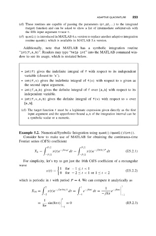
Example 5.2. Numerical/Symbolic Integration using quad()/quadl()/int().
Consider how to make use of MATLAB for obtaining the continuous-time
Fourier series (CtFS) coefficient

P/2 P/2
X k = x(t)e −jkω 0 t dt = x(t)e −j2πkt/P dt (E5.2.1)
−P/2 −P/2
For simplicity, let’s try to get just the 16th CtFS coefficient of a rectangular
wave

1 for − 1 ≤ t< 1
x(t) = (E5.2.2)
0 for − 2 ≤ t< 1or1 ≤ t< 2
which is periodic in t with period P = 4. We can compute it analytically as
1
2 1 1
−j2π16t/4 −j8πt
X 16 = x(t)e dt = e dt = e −j8πt
−2 −1 −j8π −1
1 1
= sin(8πt) = 0 (E5.2.3)
8π
−1