Page 240 - Applied Numerical Methods Using MATLAB

RECURSIVE RULE AND ROMBERG INTEGRATION 229
replacing h by h/2 in this equation yields

2
h 2 I T 2 (a,b,h/2) − I T 2 (a,b,h)
I T 4 a, b, =
2
2 2 − 1
which can be generalized to the following formula:
2n
−k
2 I T,2n (a, b, 2 −(k+1) h) − I T,2n (a, b, 2 h)
−(k+1)
I T,2(n+1) (a, b, 2 h) =
2 2n − 1
for n ≥ 1,k ≥ 0 (5.7.3)
Now, it is time to introduce a systematic way, called Romberg integration, of
improving the accuracy of the integral step by step and estimating the (trun-
cation) error at each step to determine when to stop. It is implemented by
a Romberg Table (Table 5.4), that is, a lower-triangular matrix that we con-
struct one row per iteration by applying Eq. (5.7.1) in halving the segment width
h to get the next-row element (downward in the first column), and applying
Eq. (5.7.3) in upgrading the order of error to get the next-column elements
(rightward in the row) based on the up–left (north–west) one and the left
(west) one. At each iteration k, we use Eq. (5.5.14) to estimate the truncation
error as

1

−k −k
h)
E T,2(k+1) (2 h) ≈ I T,2k (2 h) − I T,2k (2 −(k−1) (5.7.4)

2k
2 − 1
and stop the iteration when the estimated error becomes less than some prescribed
tolerance. Then, the last diagonal element is taken to be ‘supposedly’ the best
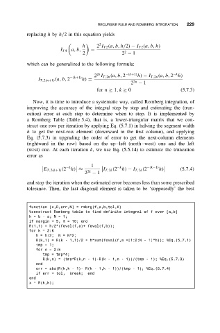
function [x,R,err,N] = rmbrg(f,a,b,tol,K)
%construct Romberg table to find definite integral of f over [a,b]
h=b-a;N=1;
if nargin < 5, K = 10; end
R(1,1) = h/2*(feval(f,a)+ feval(f,b));
for k = 2:K
h = h/2; N = N*2;
R(k,1) = R(k - 1,1)/2 + h*sum(feval(f,a +[1:2:N - 1]*h)); %Eq.(5.7.1)
tmp=1;
for n = 2:k
tmp = tmp*4;
R(k,n) = (tmp*R(k,n - 1)-R(k - 1,n - 1))/(tmp - 1); %Eq.(5.7.3)
end
err = abs(R(k,k - 1)- R(k - 1,k - 1))/(tmp - 1); %Eq.(5.7.4)
if err < tol, break; end
end
x = R(k,k);