Page 242 - Applied Numerical Methods Using MATLAB

ADAPTIVE QUADRATURE 231
one with the same number of segments N = 80. Moreover, Romberg integration
with N = 32 shows a better result than both of them.

5.8 ADAPTIVE QUADRATURE

The numerical integration methods in the previous sections divide the inte-
gration interval uniformly into the segments of equal width, making the error
nonuniform over the interval—that is, small/large for smooth/swaying portion
of the curve of integrand f(x). In contrast, the strategy of the adaptive quadra-
ture is to divide the integration interval nonuniformly into segments of (gener-
ally) unequal lengths—that is, short/long segments for swaying/smooth portion
of the curve of integrand f(x), aiming at having smaller error with fewer
segments.
The algorithm of adaptive quadrature scheme starts with a numerical integral
(INTf) for the whole interval and the sum of numerical integrals (INTf12 =
INTf1 + INTf2) for the two segments of equal width. Based on the difference
between the two successive estimates INTf and INTf12, it estimates the error of
INTf12 by using Eq. (5.5.13)/(5.5.14) depending on the basic integration rule.
Then, if the error estimate is within a given tolerance (tol), it terminates with
INTf12. Otherwise, it digs into each segment by repeating the same procedure
with half of the tolerance (tol/2) assigned to both segments, until the deepest
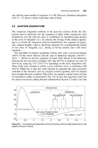
level satisfies the error condition. This is how the adaptive scheme forms sections
of nonuniform width, as illustrated in Fig. 5.4. In fact, this algorithm really fits
the nested (recursive) calling structure introduced in Section 1.3 and is cast into

whole interval
40
sub interval sub interval
30 sub-sub interval sub-sub interval

20
10

0
the curve of target function
−10 to be integrated −2x
f(x) = 400x(1 − x)e
−20
0 0.5 1 1.5 2 2.5 3 3.5 4
Figure 5.4 The subintervals (segments) and their boundary points (nodes) determined by the
adaptive Simpson method.