Page 226 - Applied Numerical Methods Using MATLAB

APPROXIMATION ERROR OF FIRST DERIVATIVE 215

10 0 0
10
10 −2
−5
10
10 −4
10 −6
10 −10
−8 h : optimal value h : optimal value
o
o
10 K 1 2e K 2 2
D (x, h) − f ′(x ) ≤ 2e + h D (x, h) − f ′(x ) ≤ + h
c2
f1
h 2 2h 6
10 −10 h o h 10 0 10 −10 h o h 10 0
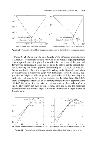
(a) Error bound of Eq. (5.1.4) vs. step size h (b) Error bound of Eq. (5.1.8) vs. step size h
Figure 5.1 Forward/central difference approximation error of first derivative versus step size h.
Figure 5.1a/b shows how the error bounds of the difference approximations
(5.1.4)/(5.1.8) for the first derivative vary with the step-size h, implying that there
is some optimal value of step-size h with which the error bound of the numerical
derivative is minimized. It seems that we might be able to get the optimal step-
size h o by using this kind of graph or directly using Eq. (5.2.2),(5.2.3) or (5.2.4).
But, as mentioned before, it is not possible, as long as the high-order derivatives
are unknown (as is usually the case). Very fortunately, Tables 5.1 and 5.2 sug-
gest that we might be able to guess the good value of h by watching how
small |D ik − D i(k−1) | is for a given problem. On the other hand, Fig. 5.2a/b
shows the tangential lines based on the forward/central difference approximations
(5.1.4)/(5.1.8) of the first derivative at x = π/4 with the three values of step-
size h. They imply that there is some optimal step-size h o and the numerical
approximation error becomes larger if we make the step-size h larger or smaller
than the value.

−8
−16 h = 10 h = 1
1 h = 10 1 h = 10 −5
f (x) = sin x f (x) = sin x
0.8 h = 0.5 0.8 h = 10 −16

0.6 0.6

0.4 0.4

0.2 0.2
0 0.5 1 1.5 x 2 0 0.5 1 1.5 x 2
(a) Forward difference approximation by Eq. (5.1.4) (b) Central difference approximation by Eq. (5.1.8)
Figure 5.2 Forward/central difference approximation of first derivative of f(x) = sin x.