Page 442 - Applied Numerical Methods Using MATLAB

GUI OF MATLAB FOR SOLVING PDES: PDETOOL 431
with boundary conditions like Eq. (9.5.2) and, additionally, the initial conditions

u(t 0 )/u (t 0 ).
4. Eigenmode PDE

−∇ · (c∇u) + au = λdu (9.5.7)

over a domain and for an unknown eigenvalue λ

with some boundary conditions like Eq. (9.5.2).

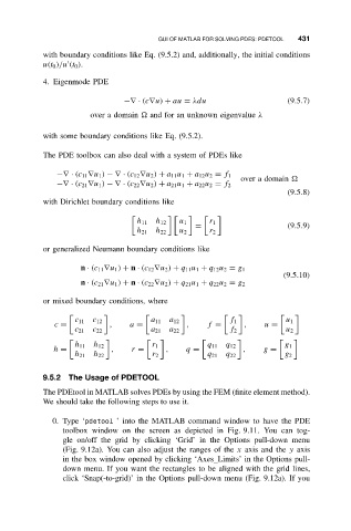
The PDE toolbox can also deal with a system of PDEs like

−∇ · (c 11 ∇u 1 ) −∇ · (c 12 ∇u 2 ) + a 11 u 1 + a 12 u 2 = f 1
over a domain
−∇ · (c 21 ∇u 1 ) −∇ · (c 22 ∇u 2 ) + a 21 u 1 + a 22 u 2 = f 2
(9.5.8)
with Dirichlet boundary conditions like

h 11 h 12 u 1 r 1
= (9.5.9)
h 21 h 22 u 2 r 2
or generalized Neumann boundary conditions like

n · (c 11 ∇u 1 ) + n · (c 12 ∇u 2 ) + q 11 u 1 + q 12 u 2 = g 1
(9.5.10)
n · (c 21 ∇u 1 ) + n · (c 22 ∇u 2 ) + q 21 u 1 + q 22 u 2 = g 2

or mixed boundary conditions, where

c 11 c 12 a 11 a 12 f 1 u 1
c = , a = , f = , u =
c 21 c 22 a 21 a 22 f 2 u 2

h 11 h 12 r 1 q 11 q 12 g 1
h = , r = , q = , g =
h 21 h 22 r 2 q 21 q 22 g 2
9.5.2 The Usage of PDETOOL
The PDEtool in MATLAB solves PDEs by using the FEM (finite element method).
We should take the following steps to use it.

0. Type ‘pdetool ’ into the MATLAB command window to have the PDE
toolbox window on the screen as depicted in Fig. 9.11. You can tog-
gle on/off the grid by clicking ‘Grid’ in the Options pull-down menu
(Fig. 9.12a). You can also adjust the ranges of the x axis and the y axis
in the box window opened by clicking ‘Axes Limits’ in the Options pull-
down menu. If you want the rectangles to be aligned with the grid lines,
click ‘Snap(-to-grid)’ in the Options pull-down menu (Fig. 9.12a). If you