Page 438 - Applied Numerical Methods Using MATLAB

FINITE ELEMENT METHOD (FEM) FOR SOLVING PDE 427
Example 9.6. Laplace’s Equation: Electric Potential Over a Plate with Point
Charge. Consider the following Laplace’s equation:
2
2
∂ u(x, y) ∂ u(x, y)
2
∇ u(x, y) = + = f (x, y) (E9.6.1)
∂x 2 ∂y 2
for − 1 ≤ x ≤+1, −1 ≤ y ≤+1
where 
 −1for (x, y) = (0.5, 0.5)
f (x, y) = +1for (x, y) = (−0.5, −0.5) (E9.6.2)
0 elsewhere

and the boundary condition is u(x, y) = 0 for all boundaries of the rectangu-
lar domain.
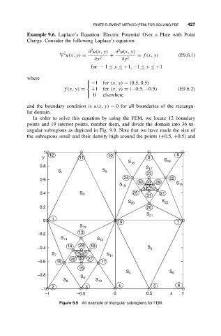
In order to solve this equation by using the FEM, we locate 12 boundary
points and 19 interior points, number them, and divide the domain into 36 tri-
angular subregions as depicted in Fig. 9.9. Note that we have made the size of
the subregions small and their density high around the points (+0.5, +0.5) and

1
y 12 11 10 9 8
S 18 S 16
0.8 S 17
S 1 S 3 23
24 22
0.6
S 19 30 33 29 S 15
36
34 32
0.4 S 2 25 31 21
S 20 S 22
0.2 20
S 21
0 1 19 7
S 13
−0.2 13
S 14 S 12
−0.4 14 28 18 S 5
S 29 31
7 35 S 11
26 30 27
−0.6 15 17
16
S 4 S 6
−0.8 S
S 8 9 S 10
−1 2 3 4 5 6
−1 −0.5 0 0.5 x 1

Figure 9.9 An example of triangular subregions for FEM.