Page 436 - Applied Numerical Methods Using MATLAB

FINITE ELEMENT METHOD (FEM) FOR SOLVING PDE 425

1 1

0.5 0.5
(0.2, 0.5)
0 0
1 1 1 1
0 0 0 0
−1 −1 −1 −1
(a) f (x, y) (b) f (x, y )
2
1

1 1

0.5 0.5

0 0
1 1 1
1
0 0 0 0
−1 −1 −1 −1
(x, y ) (x, y )
(c) f 3 (d) f 4

1 4

0.5 2

0 0
1 1
1 1
0 0 0 0
−1 −1 −1 −1
(x,y ) (x, y )+2f (x, y)+3f (x, y)
(e) f 5 (f) f 2 3 4
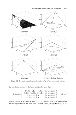
Figure 9.8 The basis (shape) functions for nodes in Fig. 9.7 and a composite function.

the coefficient vectors of the basis function for node 2 as


 −7/10 + (1/2)x + (6/5)y for subregion S 1

−7/16 + (15/16)x + (1/2)y for subregion S 2

φ 2 (x, y) = (9.4.18)
0 + 0 · x + 0 · y for subregion S 3


0 + 0 · x + 0 · y for subregion S 4

which turns out to be 1 only at node 2 [i.e., (1,1)] and 0 at all other nodes and on
the subregions that do not have node 2 as their vertex, as depicted in Fig. 9.8b.