Page 435 - Applied Numerical Methods Using MATLAB

424 PARTIAL DIFFERENTIAL EQUATIONS
1
n = 1 n = 2 coordinates of
S 1 nodes
N = [−1 1;
0.5 n = 5 1 1;
1 −1;
S 2
S 4
−1 −1;
0.2 0.5]
0
node numbers
of subregions
S 3
−0.5 S = [1 2 5;
2 3 5;
3 4 5;
n = 4 1 4 5]
−1 n = 3
−1 −0.5 0 0.5 1
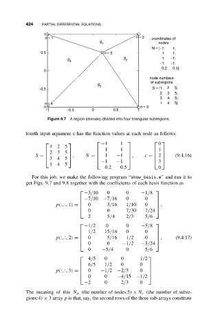
Figure 9.7 A region (domain) divided into four triangular subregions.

fourth input argument c has the function values at each node as follows:

   
  −1 1 0
125
 1
 235  1   1 
 


S =   , N =  1 −1  , c =  2  (9.4.16)
 345 
−1 −1 3
   
145
0.2 0.5 0
For this job, we make the following program “show_basis.m”and runit to
get Figs. 9.7 and 9.8 together with the coefficients of each basis function as
−3/10 0 0 −1/8
 
 −7/10 −7/16 0 0 
p(:, :, 1) =  0 3/16 1/10 0  ,


0 0 7/30 7/24
 
2 5/4 2/3 5/6
−1/2 0 0 −5/8
 
 1/2 15/16 0 0 
p(:, :, 2) =  0 5/16 1/2 0  , (9.4.17)


0 0 −1/2 −5/24
 
0 −5/4 0 5/6
4/5 0 0 1/2
 
 6/5 1/2 0 0 
p(:, :, 3) =  0 −1/2 −2/5 0 


0 0 −4/15 −1/2
 
−2 0 2/3 0
The meaning of this N n (the number of nodes:5) × N s (the number of subre-
gions:4) × 3 array p is that, say, the second rows of the three sub-arrays constitute