Page 439 - Applied Numerical Methods Using MATLAB

428 PARTIAL DIFFERENTIAL EQUATIONS
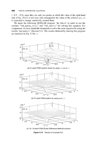
(−0.5, −0.5), since they are only two points at which the value of the right-hand
side of Eq. (9.6.1) is not zero, and consequently the value of the solution u(x, y)
is expected to change sensitively around them.
We made the following MATLAB program “do_fem.m” in order to use the
routines “fem_basis_ftn()”and “fem_coef()” for solving this equation. For
comparison, we have added the statements to solve the same equation by using the
routine “poisson()” (Section 9.1). The results obtained by running this program
are depicted in Fig. 9.10a–c.

x10 −3
5
u(x, y)
0

−5
1
y 1
0.5 x
0 0 0.5
−0.5 −0.5
−1 −1
(a) 31-point FEM solution drawn by using trimesh ()

x10 −3
5
u(x, y)
0

−5
1
y
0.5 x 1
0 0.5
−0.5 −0.5 0
−1 −1
(b) 31-point FEM solution by using mesh ()

x10 −3
5
u(x, y)
0

−5
1
y 1
0.5 x
0 0 0.5
−0.5 −0.5
−1 −1
(c) 16×15-point FDM (Finite Difference Method) solution
Figure 9.10 Results of Example 9.6.