Page 434 - Applied Numerical Methods Using MATLAB

FINITE ELEMENT METHOD (FEM) FOR SOLVING PDE 423

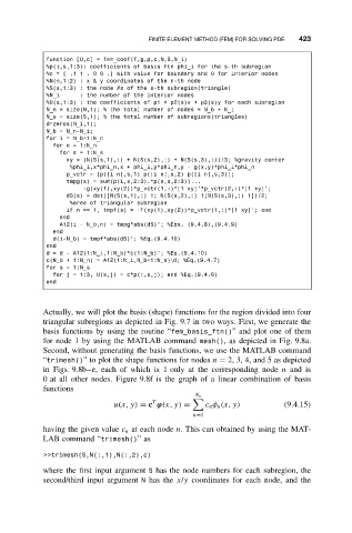
function [U,c] = fem_coef(f,g,p,c,N,S,N_i)
%p(i,s,1:3): coefficients of basis ftn phi_i for the s-th subregion
%c=[.11.00.] with value for boundary and 0 for interior nodes
%N(n,1:2):x&y coordinates of the n-th node
%S(s,1:3) : the node #s of the s-th subregion(triangle)
%N_i : the number of the interior nodes
%U(s,1:3) : the coefficients of p1 + p2(s)x + p3(s)y for each subregion
N_n = size(N,1); % the total number of nodes = N_b + N_i
N_s = size(S,1); % the total number of subregions(triangles)
d=zeros(N_i,1);
N_b = N_n-N_i;
for i = N_b+1:N_n
for n = 1:N_n
for s = 1:N_s
xy = (N(S(s,1),:) + N(S(s,2),:) + N(S(s,3),:))/3; %gravity center
%phi_i,x*phi_n,x + phi_i,y*phi_n,y - g(x,y)*phi_i*phi_n
p_vctr = [p([i n],s,1) p([i n],s,2) p([i n],s,3)];
tmpg(s) = sum(p(i,s,2:3).*p(n,s,2:3))...
-g(xy(1),xy(2))*p_vctr(1,:)*[1 xy]’*p_vctr(2,:)*[1 xy]’;
dS(s) = det([N(S(s,1),:) 1; N(S(s,2),:) 1;N(S(s,3),:) 1])/2;
%area of triangular subregion
if n == 1, tmpf(s) = -f(xy(1),xy(2))*p_vctr(1,:)*[1 xy]’; end
end
A12(i - N_b,n) = tmpg*abs(dS)’; %Eqs. (9.4.8),(9.4.9)
end
d(i-N_b) = tmpf*abs(dS)’; %Eq.(9.4.10)
end
d=d- A12(1:N_i,1:N_b)*c(1:N_b)’; %Eq.(9.4.10)
c(N_b + 1:N_n) = A12(1:N_i,N_b+1:N_n)\d; %Eq.(9.4.7)
for s = 1:N_s
for j = 1:3, U(s,j) = c*p(:,s,j); end %Eq.(9.4.6)
end

Actually, we will plot the basis (shape) functions for the region divided into four
triangular subregions as depicted in Fig. 9.7 in two ways. First, we generate the
basis functions by using the routine “fem_basis_ftn()” and plot one of them
for node 1 by using the MATLAB command mesh(), as depicted in Fig. 9.8a.
Second, without generating the basis functions, we use the MATLAB command
“trimesh()” to plot the shape functions for nodes n = 2, 3, 4, and 5 as depicted
in Figs. 9.8b–e, each of which is 1 only at the corresponding node n and is
0 at all other nodes. Figure 9.8f is the graph of a linear combination of basis
functions
N n
T
u(x, y) = c ϕ(x, y) = c n φ n (x, y) (9.4.15)
n=1
having the given value c n at each node n. This can obtained by using the MAT-
LAB command “trimesh()”as

>>trimesh(S,N(:,1),N(:,2),c)
where the first input argument S has the node numbers for each subregion, the
second/third input argument N has the x/y coordinates for each node, and the