Page 486 - Applied Numerical Methods Using MATLAB

APPENDIX E

FOURIER TRANSFORM

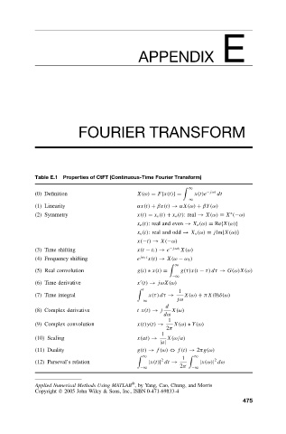
Table E.1 Properties of CtFT (Continuous-Time Fourier Transform)
∞

(0) Definition X(ω) = F{x(t)}= x(t)e −jωt dt
−∞
(1) Linearity αx(t) + βx(t) → αX(ω) + βY(ω)
(2) Symmetry x(t) = x e (t) + x o (t): real → X(ω) ≡ X (−ω)
∗
x e (t): real and even → X e (ω) = Re{X(ω)}
x o (t): real and odd → X o (ω) = jIm{X(ω)}
x(−t) → X(−ω)
(3) Time shifting x(t − t 1 ) → e −jωt 1 X(ω)
(4) Frequency shifting e jω 1 t x(t) → X(ω − ω 1 )
∞

(5) Real convolution g(t) ∗ x(t) = g(τ)x(t − τ) dτ → G(ω)X(ω)
−∞
(6) Time derivative x (t) → jωX(ω)

t 1
(7) Time integral x(τ) dτ → X(ω) + πX(0)δ(ω)
jω
−∞
d
(8) Complex derivative tx(t) → j X(ω)
dω
1
(9) Complex convolution x(t)y(t) → X(ω) ∗ Y(ω)
2π
1
(10) Scaling x(at) → X(ω/a)
|a|
(11) Duality g(t) → f(ω) ⇔ f(t) → 2πg(ω)
∞ 1 ∞

2
2
(12) Parseval’s relation |x(t)| dt → |x(ω)| dω
2π
−∞ −∞

Applied Numerical Methods Using MATLAB , by Yang, Cao, Chung, and Morris
Copyright  2005 John Wiley & Sons, I nc., ISBN 0-471-69833-4

475