Page 162 - Applied Probability

8. The Polygenic Model
that the hypothesis σ = 0 is equivalent to the hypothesis ρ frat = ρ ident.
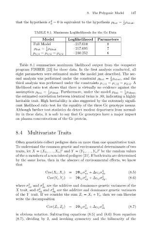
TABLE 8.1. Maximum Loglikelihoods for the Gc Data
Model
- 217.610
8
Full Model 2 d Loglikelihood Parameters 1 2 147
1
ρ frat = ρ ident - 217.695 7
2
- 230.252 6
µ 1/1 = µ 1/2 = µ 2/2
Table 8.1 summarizes maximum likelihood output from the computer
program FISHER [22] for these data. In the first analysis conducted, all
eight parameters were estimated under the model just described. The sec-
1
ond analysis was performed under the constraint ρ frat = ρ ident, and the
2
third analysis was performed under the constraints µ 1/1 = µ 1/2 = µ 2/2 .A
likelihood ratio test shows that there is virtually no evidence against the
1
1
assumption ρ frat = ρ ident. Furthermore, under the model ρ frat = ρ ident,
2 2
the estimated correlation between identical twins is .80, indicating a highly
heritable trait. High heritability is also suggested by the extremely signifi-
cant likelihood ratio test for the equality of the three Gc genotype means.
Although further test statistics do detect modest departures from normal-
ity in these data, it is safe to say that Gc genotypes have a major impact
on plasma concentrations of the Gc protein.
8.4 Multivariate Traits
Often geneticists collect pedigree data on more than one quantitative trait.
To understand the common genetic and environmental determinants of two
t
t
traits, let X =(X 1 ,...,X n ) and Y =(Y 1 ,...,Y n ) be the random values
of the n members of a non-inbred pedigree [21]. If both traits are determined
by the same locus, then in the absence of environmental effects, we know
that
2
Cov(X i ,X j )=2Φ ij σ 2 ax +∆ 7ij σ dx (8.5)
2
Cov(Y i ,Y j )=2Φ ij σ 2 ay +∆ 7ij σ , (8.6)
dy
where σ 2 and σ 2 are the additive and dominance genetic variances of the
ax dx
X trait, and σ 2 and σ 2 are the additive and dominance genetic variances
ay dy
of the Y trait. If we consider the sum Z i = X i + Y i , then we can likewise
write the decomposition
Cov(Z i ,Z j )=2Φ ij σ 2 az +∆ 7ij σ 2 dz (8.7)

in obvious notation. Subtracting equations (8.5) and (8.6) from equation
(8.7), dividing by 2, and invoking symmetry and the bilinearity of the