Page 163 - Applied Probability

148
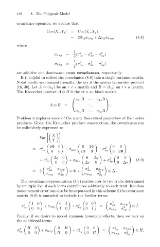
covariance operator, we deduce that
Cov(X i ,Y j )=Cov(Y i ,X j )
where 8. The Polygenic Model =2Φ ij σ axy +∆ 7ij σ dxy , (8.8)
1 2 2 2
= (σ − σ − σ )
σ axy az ax ay
2
1 2 2 2
= (σ − σ − σ )
σ dxy dz dx dy
2
are additive and dominance cross covariances, respectively.
It is helpful to collect the covariances (8.8) into a single variance matrix.
Notationally and computationally, the key is the matrix Kronecker product
[16, 30]. Let A =(a ij )bean r × s matrix and B =(b ij )an t × u matrix.
The Kronecker product A ⊗ B is the rt × su block matrix
a 11 B ··· a 1s B
 
. . .
A ⊗ B =  . . . . . .  .
a r1 B ··· a rs B
Problem 8 explores some of the many theoretical properties of Kronecker
products. Given the Kronecker product construction, the covariances can
be collectively expressed as

ø
X
Var
Y

2Φ 0 0 2Φ 2 0 0
2
= σ ax + σ axy + σ ay
0 0 2Φ 0 02Φ

+ σ 2 dx ∆ 7 0 + σ dxy 0 ∆ 7 + σ 2 dy 0 0 (8.9)
0 0 ∆ 7 0 0∆ 7
2 2
σ ax σ axy σ σ dxy
=2 2 ⊗ Φ+ dx 2 ⊗ ∆ 7 .
σ axy σ ay σ dxy σ dy
The covariance representation (8.9) carries over to two traits determined
by multiple loci if each locus contributes additively to each trait. Random
measurement error can also be incorporated in this scheme if the covariance
matrix (8.9) is amended to include the further terms
2
I 0 0 I 2 00 σ ex σ exy
2
σ ex + σ exy + σ ey = 2 ⊗ I.
0 0 I 0 0 I σ exy σ ey
Finally, if we desire to model common household effects, then we tack on
the additional terms
2
H 0 0 H 2 0 0 σ σ hxy
2
σ hx + σ hxy + σ hy = hx 2 ⊗ H,
0 0 H 0 0 H σ hxy σ
hy