Page 166 - Applied Probability

8. The Polygenic Model
151
model where σ
lihoods produces a lod score similar to the classical lod score of linkage
analysis. Twice the difference in log likelihoods of these two models yields
e
a test statistic that is asymptotically distributed as a 1/2: 1/2 mixture
of a χ variable and a point mass at zero [33]. When multiple QTLs are
1 2 2 ai is estimated. The difference between the two log 10 like-
jointly considered, the resulting likelihood ratio test statistic has a more
complicated asymptotic distribution. Accurate computation of the condi-
ˆ
tional kinship matrices Φ i as a function of map position of the ith QTL
is obviously a critical step in QTL mapping. Fortunately, this problem can
be attacked by exact computation on small pedigrees and stochastic sim-
ulation methods on large pedigrees. We defer discussion of particulars to
Chapter 9.
8.7 Factor Analysis
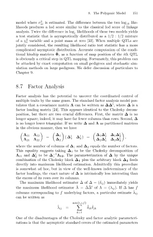
Factor analysis has the potential to uncover the coordinated control of
multiple traits by the same genes. The standard factor analysis model pos-
t
tulates that a covariance matrix Λ can be written as ∆∆ , where ∆ is a
factor loading matrix [24]. This appears identical to the Cholesky decom-
position, but there are two crucial differences. First, the matrix ∆ is no
longer square; indeed, it may have far fewer columns than rows. Second, ∆
is no longer lower triangular. If we write ∆ and Λ as partitioned matrices
in the obvious manner, then we have
t t
Λ 11 Λ 12 ∆ 1 t t ∆ 1 ∆ 1 ∆ 1 ∆ 2
= ( ∆ 1 ∆ )= t t ,
2
Λ 21 Λ 22 ∆ 2 ∆ 2 ∆ ∆ 2 ∆
1 2
where the number of columns of ∆ 1 and ∆ 2 equals the number of factors.
This equality suggests taking ∆ 1 to be the Cholesky decomposition of
t
Λ 11 and ∆ to be ∆ −1 Λ 12. The parameterization of ∆ by the unique
2 1
combination of the Cholesky block ∆ 1 plus the arbitrary block ∆ 2 feeds
directly into maximum likelihood estimation. Admittedly this procedure
is somewhat ad hoc, but in view of the well-known indeterminacy of the
factor loadings, the exact nature of ∆ is intrinsically less interesting than
the excess of its rows over its columns.
ˆ
The maximum likelihood estimator ∆of ∆ = (δ ij ) immediately yields
ˆ
ˆ ˆ t
the maximum likelihood estimator Λ= ∆∆ of Λ = (λ ij ). If ∆ has f
ˆ
columns corresponding to f underlying factors, a particular estimate λ ij
can be written as
min{i,j,f}
ˆ ˆ ˆ
λ ij = δ ik δ jk
k=1
One of the disadvantages of the Cholesky and factor analytic parameteri-
zations is that the asymptotic standard errors of the estimated parameters