Page 164 - Applied Probability

8. The Polygenic Model
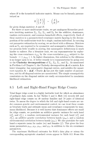
where H is the household indicator matrix. Means can be linearly parame-
terized as

ø

X
E
Y
B
for given design matrices A and B. = A µ 149
For three or more multivariate traits, we get analogous Kronecker prod-
ucts involving matrices Σ a ,Σ d ,Σ e , and Σ h for the additive, dominance,
random environment, and common household effects, respectively. Each of
these matrices is a parameterized covariance matrix figuring in the decom-
position of the multivariate trait for a single, random individual. In carrying
out parameter estimation by scoring, we are faced with a dilemma. Matrices
such as Σ a are required to be symmetric and nonnegative definite. Symme-
try presents little trouble in scoring, but nonnegative definiteness is much
harder to enforce. For a bivariate trait, we can reparameterize by replac-
ing the cross-covariance σ axy by the cross-correlation ρ axy subject to the
bounds −1 ≤ ρ axy ≤ 1. In higher dimensions, this solution to the dilemma
is no longer open to us. A better remedy is to reparameterize by going over
to the Cholesky decompositions of Σ a ,Σ d,Σ e , and Σ h . As mentioned
in Problem 4 of Chapter 5, the Cholesky decomposition ∆ of a matrix Λ is
lower triangular, has nonnegative diagonal entries, and satisfies the square
t
root equation Λ = ∆∆ . Clearly ∆ has just the right number of parame-
ters, and its off-diagonal entries are unrestricted. The simple nonnegativity
constraints on the diagonal entries are easily accommodated in maximum
likelihood estimation.

8.5 Left and Right-Hand Finger Ridge Counts

Total finger ridge count is a highly heritable trait for which an abundance
of pedigree data exists. In her Tables 1 and 3, Holt [14] records left and
right-hand ridge counts on 48 nuclear families and 18 pairs of identical
twins. To assess the degree to which the left and right-hand counts are un-
der common genetic and environmental control, we can treat these counts
as bivariate traits and estimate mean and covariance components by max-
imum likelihood. Because it is well known that dominance effects are small
for ridge counts, we postulate an additive genetic variance for each hand
2
(σ 2 al and σ ), a random environmental variance for each hand (σ 2 el and
ar
2
σ ), an additive genetic correlation between hands (ρ alr ), and a random
er
environmental correlation between hands (ρ elr ). We also postulate for each
hand a separate mean for males (m) and females (f). This gives the four
mean parameters µ ml , µ fl , µ mr , and µ fr in addition to the six covariance
parameters.
The maximum likelihood estimates for Holt’s data plus or minus the
corresponding asymptotic standard errors appear in Table 8.2. From this