Page 132 - Applied Statistics And Probability For Engineers

c04.qxd 5/13/02 11:17 M Page 110 RK UL 6 RK UL 6:Desktop Folder:TEMP WORK:MONTGOMERY:REVISES UPLO D CH114 FIN L:Quark Files:

110 CHAPTER 4 CONTINUOUS RANDOM VARIABLES AND PROBABILITY DISTRIBUTIONS

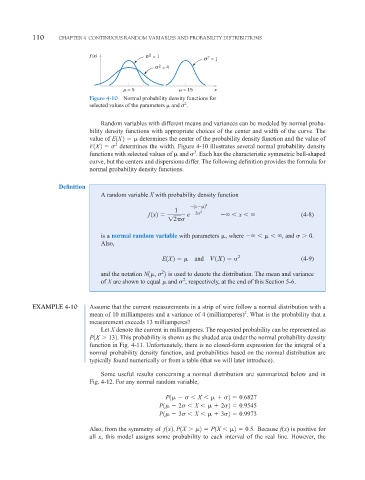
f (x) σ 2 = 1
σ 2 = 1
σ 2 = 4

= 5 = 15 x
Figure 4-10 Normal probability density functions for
2

selected values of the parameters and .
Random variables with different means and variances can be modeled by normal proba-
bility density functions with appropriate choices of the center and width of the curve. The
value of E1X2 determines the center of the probability density function and the value of
V1X2 2 determines the width. Figure 4-10 illustrates several normal probability density
2
functions with selected values of and . Each has the characteristic symmetric bell-shaped
curve, but the centers and dispersions differ. The following definition provides the formula for
normal probability density functions.

Definition
A random variable X with probability density function
1x 2 2
1 2
f 1x2 e 2 x (4-8)
12

is a normal random variable with parameters , where , and 0.
Also,
E1X2 and V1X2 2 (4-9)

2
and the notation N1 , 2 is used to denote the distribution. The mean and variance
2
of X are shown to equal and , respectively, at the end of this Section 5-6.

EXAMPLE 4-10 Assume that the current measurements in a strip of wire follow a normal distribution with a
2
mean of 10 milliamperes and a variance of 4 (milliamperes) . What is the probability that a
measurement exceeds 13 milliamperes?
Let X denote the current in milliamperes. The requested probability can be represented as
P1X 132. This probability is shown as the shaded area under the normal probability density
function in Fig. 4-11. Unfortunately, there is no closed-form expression for the integral of a
normal probability density function, and probabilities based on the normal distribution are
typically found numerically or from a table (that we will later introduce).
Some useful results concerning a normal distribution are summarized below and in
Fig. 4-12. For any normal random variable,

P1 X
2 0.6827
P1 2 X
2 2 0.9545
P1 3 X
3 2 0.9973

Also, from the symmetry of f 1x2, P1X 2 P1X 2 0.5. Because f(x) is positive for
all x, this model assigns some probability to each interval of the real line. However, the