Page 134 - Applied Statistics And Probability For Engineers

c04.qxd 5/10/02 5:19 PM Page 112 RK UL 6 RK UL 6:Desktop Folder:TEMP WORK:MONTGOMERY:REVISES UPLO D CH114 FIN L:Quark Files:

112 CHAPTER 4 CONTINUOUS RANDOM VARIABLES AND PROBABILITY DISTRIBUTIONS

P(Z ≤ 1.5) = Φ(1.5)
z 0.00 0.01 0.02 0.03
= shaded area
0 0.50000 0.50399 0.50398 0.51197
Figure 4-13 Standard . . . . . .
normal probability den-
1.5 0.93319 0.93448 0.93574 0.93699
sity function. 0 1.5 z
Probabilities that are not of the form P(Z z ) are found by using the basic rules of prob-
ability and the symmetry of the normal distribution along with Appendix Table II. The fol-
lowing examples illustrate the method.
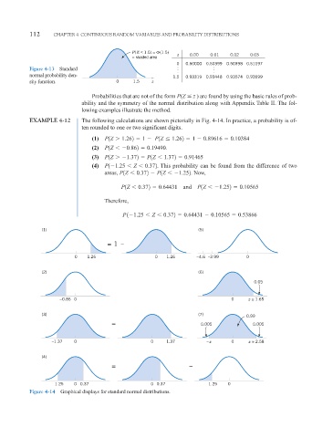
EXAMPLE 4-12 The following calculations are shown pictorially in Fig. 4-14. In practice, a probability is of-
ten rounded to one or two significant digits.

(1) P1Z 1.262 1 P1Z 1.262 1 0.89616 0.10384
(2) P1Z 0.862 0.19490.
(3) P1Z 1.372 P1Z 1.372 0.91465
(4) P1 1.25 Z 0.372 . This probability can be found from the difference of two
areas, P1Z 0.372 P1Z 1.252 . Now,

P1Z 0.372 0.64431 and P1Z 1.252 0.10565

Therefore,

P 1 1.25 Z 0.372 0.64431 0.10565 0.53866

(1) (5)

= 1 –

0 1.26 0 1.26 –4.6 –3.99 0

(2) (6)

0.05

–0.86 0 0 z ≅ 1.65

(3) (7)
0.99
= 0.005 0.005

–1.37 0 0 1.37 – z 0 z ≅ 2.58

(4)
= –

–1.25 0 0.37 0 0.37 –1.25 0
Figure 4-14 Graphical displays for standard normal distributions.