Page 138 - Applied Statistics And Probability For Engineers

c04.qxd 5/10/02 5:19 PM Page 116 RK UL 6 RK UL 6:Desktop Folder:TEMP WORK:MONTGOMERY:REVISES UPLO D CH114 FIN L:Quark Files:

116 CHAPTER 4 CONTINUOUS RANDOM VARIABLES AND PROBABILITY DISTRIBUTIONS

Therefore,

x 0.45 2.58

and

x 2.5810.452 1.16

Suppose a digital 1 is represented as a shift in the mean of the noise distribution to 1.8
volts. What is the probability that a digital 1 is not detected? Let the random variable S denote
the voltage when a digital 1 is transmitted. Then,

S 1.8 0.9 1.8
P1S 0.92 P a b P1Z 22 0.02275
0.45 0.45

This probability can be interpreted as the probability of a missed signal.

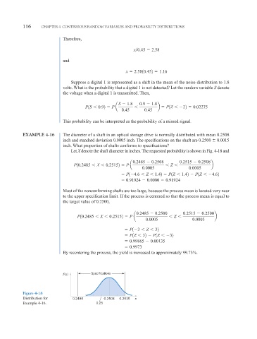
EXAMPLE 4-16 The diameter of a shaft in an optical storage drive is normally distributed with mean 0.2508
inch and standard deviation 0.0005 inch. The specifications on the shaft are 0.2500 0.0015
inch. What proportion of shafts conforms to specifications?
Let X denote the shaft diameter in inches. The requested probability is shown in Fig. 4-18 and

0.2485 0.2508 0.2515 0.2508
P10.2485 X 0.25152 P a Z b
0.0005 0.0005
P1 4.6 Z 1.42 P1Z 1.42 P1Z 4.62
0.91924 0.0000 0.91924

Most of the nonconforming shafts are too large, because the process mean is located very near
to the upper specification limit. If the process is centered so that the process mean is equal to
the target value of 0.2500,

0.2485 0.2500 0.2515 0.2500
P10.2485 X 0.25152 P a Z b
0.0005 0.0005

P1 3 Z 32
P1Z 32 P1Z 32
0.99865 0.00135
0.9973
By recentering the process, the yield is increased to approximately 99.73%.

f(x) Specifications

Figure 4-18
Distribution for 0.2485 0.2508 0.2515 x
Example 4-16. 0.25