Page 141 - Applied Statistics And Probability For Engineers

c04.qxd 5/10/02 5:19 PM Page 119 RK UL 6 RK UL 6:Desktop Folder:TEMP WORK:MONTGOMERY:REVISES UPLO D CH114 FIN L:Quark Files:

4-7 NORMAL APPROXIMATION TO THE BINOMIAL AND POISSON DISTRIBUTIONS 119

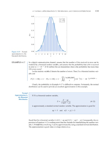
0.25
n = 10
p = 0.5
0.20

0.15

f(x)
0.10

0.05

Figure 4-19 Normal 0.00
approximation to the 0 1 2 3 4 5 6 7 8 9 10
binomial distribution. x

EXAMPLE 4-17 In a digital communication channel, assume that the number of bits received in error can be
modeled by a binomial random variable, and assume that the probability that a bit is received
in error is 1 10 5 . If 16 million bits are transmitted, what is the probability that more than
150 errors occur?
Let the random variable X denote the number of errors. Then X is a binomial random vari-
able and
150 16,000,000
5 16,000,000 x
5 x
P 1X 1502 1 P1x 1502 1 a a b 110 2 11 10 2
x 0 x
Clearly, the probability in Example 4-17 is difficult to compute. Fortunately, the normal
distribution can be used to provide an excellent approximation in this example.

Normal
Approximation to If X is a binomial random variable,
the Binomial
Distribution X np
Z (4-12)
1np11 p2
is approximately a standard normal random variable. The approximation is good for

np 5 and n11 p2 5

Recall that for a binomial variable X, E(X) np and V(X) np(1 p). Consequently, the ex-
pression in Equation 4-12 is nothing more than the formula for standardizing the random vari-
able X. Probabilities involving X can be approximated by using a standard normal distribution.
The approximation is good when n is large relative to p.