Page 136 - Applied Statistics And Probability For Engineers

c04.qxd 5/10/02 5:19 PM Page 114 RK UL 6 RK UL 6:Desktop Folder:TEMP WORK:MONTGOMERY:REVISES UPLO D CH114 FIN L:Quark Files:

114 CHAPTER 4 CONTINUOUS RANDOM VARIABLES AND PROBABILITY DISTRIBUTIONS

X – µ
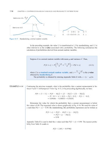
Distribution of Z =
σ

0 1.5 z
Distribution of X

4 7 9 1011 13 16 x
–3 –1.5 –0.5 0 0.5 1.5 3 z
10 13 x
Figure 4-15 Standardizing a normal random variable.

In the preceding example, the value 13 is transformed to 1.5 by standardizing, and 1.5 is
often referred to as the z-value associated with a probability. The following summarizes the
calculation of probabilities derived from normal random variables.

2
Suppose X is a normal random variable with mean and variance . Then,
X x
P 1X x2 P a b P1Z z2 (4-11)

1x 2
where Z is a standard normal random variable, and z is the z-value
obtained by standardizing X.
The probability is obtained by entering Appendix Table II with z 1x 2 .

EXAMPLE 4-14 Continuing the previous example, what is the probability that a current measurement is be-
tween 9 and 11 milliamperes? From Fig. 4-15, or by proceeding algebraically, we have

P19 X 112 P119 102 2 1X 102 2 111 102 22
P1 0.5 Z 0.52 P1Z 0.52 P1Z 0.52
0.69146 0.30854 0.38292

Determine the value for which the probability that a current measurement is below
this value is 0.98. The requested value is shown graphically in Fig. 4-16. We need the value of
x such that P(X x) 0.98. By standardizing, this probability expression can be written as

P1X x2 P11X 102 2 1x 102 22
P1Z 1x 102 22
0.98

Appendix Table II is used to find the z-value such that P(Z z) 0.98. The nearest proba-
bility from Table II results in

P1Z 2.052 0.97982